Page 452 - Automotive Engineering Powertrain Chassis System and Vehicle Body

Decisional architecture C HAPTER 14.2

Dynamic model of AA is modelled as a rigid body Equations 14.2.21 to 14.2.23 represent the forces
supported by four wheels with rigid suspensions. With- required to maintain the velocity _ s and the acceleration € s
! of A at a given position s along the path. Although simple,
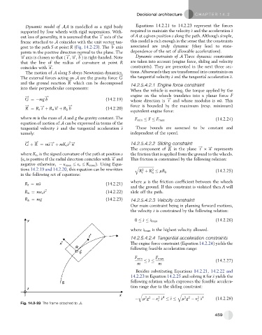
out loss of generality, it is assumed that the t axis of the
frame attached to A coincides with the unit vector tan- this model is rich enough in the sense that the constraints
!
gent to the path S at point R (Fig. 14.2-23). The b axis associated are truly dynamic (they lead to state-
points in the positive direction normal to the plane. The dependence of the set of allowable accelerations).
! ! ! ! Dynamic constraints of A Three dynamic constraints
n axis is chosen so that ð t ; n ; b Þ is right-handed. Note
that the line of the radius of curvature at point R are taken into account (engine force, sliding and velocity
!
coincides with n . constraints). They are presented in the next three sec-
The motion of A along S obeys Newtonian dynamics. tions. Afterwards they are transformed into constraints on
!
The external forces acting on A are the gravity force G the tangential velocity _ s and the tangential acceleration € s.
!
and the ground reaction R which can be decomposed 14.2.5.4.2.1 Engine force constraint
into their perpendicular components:
When the vehicle is moving, the torque applied by the
! ! engine on the wheels translates into a planar force F
!
G ¼ mg b (14.2.19) whose direction is t and whose modulus is m€ s. This
! ! ! ! force is bounded by the maximum (resp. minimum)
R ¼ R t t þ R n n þ R b (14.2.20) equivalent engine force:
b
where m is the mass of A and g the gravity constant. The F min F F max (14.2.24)
equation of motion of A can be expressed in terms of the
tangential velocity _ s and the tangential acceleration € s These bounds are assumed to be constant and
namely: independent of the speed.

! ! ! 2!
G þ R ¼ m€ st þ mK s _ s n 14.2.5.4.2.2 Sliding constraint
!
!
!
The component of R in the plane t n represents
where K s , is the signed curvature of the path at position s the friction that is applied from the ground to the wheels.
!
(k s is positive if the radial direction coincides with n and This friction is constrained by the following relation:
negative otherwise, k max k s K max ). Using Equa- q ffiffiffiffiffiffiffiffiffiffiffiffiffiffiffiffiffi
tions 14.2.19 and 14.2.20, this equation can be rewritten R þ R mR b (14.2.25)
2
2
in the following set of equations: t n
where m is the friction coefficient between the wheels
R t ¼ m€ s (14.2.21)
and the ground. If this constraint is violated then A will
R n ¼ mk s _ s 2 (14.2.22) slide off the path.
R ¼ mg (14.2.23) 14.2.5.4.2.3 Velocity constraint
b
Our main constraint being in planning forward motions,
the velocity _ s is constrained by the following relation:
0 _ s _ s max (14.2.26)
where _ s max is the highest velocity allowed.

14.2.5.4.2.4 Tangential acceleration constraints
The engine force constraint (Equation 14.2.24) yields the
following feasible acceleration range:

F min F max
€ s (14.2.27)
m m
Besides substituting Equations 14.2.21, 14.2.22 and
14.2.23 in Equation 14.2.25 and solving it for€ s yields the
following relation which expresses the feasible accelera-
tion range due to the sliding constraint:
q ffiffiffiffiffiffiffiffiffiffiffiffiffiffiffiffiffiffiffiffiffiffiffiffiffi q ffiffiffiffiffiffiffiffiffiffiffiffiffiffiffiffiffiffiffiffiffiffiffiffiffi
2 4
2 4
2 2
2 2
m g k _ s € s m g k _ s (14.2.28)
s
s
Fig. 14.2-23 The frame attached to A.
459