Page 457 - Automotive Engineering Powertrain Chassis System and Vehicle Body

CHAP TER 1 4. 2 Decisional architecture

14.2.5.5.5 Implementation and experiments
The algorithm presented earlier has been implemented
in C on a Sparc station. Two examples of trajectory
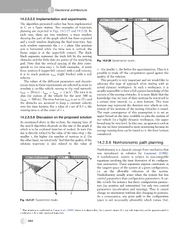
planning are depicted in Figs. 14.2-27 and 14.2-28.In
each case, there are two windows: a trace window
showing the part of the graph which has been explored
and a result window displaying the final trajectory. Any
such window represents the s t plane (the position
axis is horizontal while the time axis is vertical; the
frame origin is at the upper-left corner). The thick
black segments represent the trails left by the moving
obstacles and the little dots are points of the underlying Fig. 14.2-28 Experimental results.
grid. Note that the vertical spacing of the dots corre-
sponds to the time-step s. In both examples, A starts
from position 0 (upper-left corner) with a null velocity, s – the smaller s, the better the approximation. Thus it is
it is to reach position s max (right border) with a null possible to trade off the computation speed against the
velocity. quality of the solution.
The values of the different parameters and discreti- This property is very important and we would like to
zation steps in these experiments are selected in order to advocate this type of approach when dealing with an
simulate a car-like vehicle moving in the road network: actual dynamic workspace. In such a workspace, it is
2
_ s max ¼ 20 m=s € s min ¼ € s max ¼ 1m=s . The idea is to usually impossible to have a full a priori knowledge of the
plan the motion of the vehicle for the next 500 m motion of the moving obstacles. It is more likely that the
ðs max ¼ 500 mÞ. The time horizon t max is set to 25 s and knowledge that we have of their motions be restricted to
the obstacles are assumed to keep a constant velocity a certain time interval, i.e. a time horizon. This time
over the time horizon. For a value of s set of 0.5 s, the horizon may represent the duration over which an esti-
running time is of the order of 1 s. mation of the motions of the moving obstacles is sound.
The main consequence of this assumption is to set an
upper bound on the time available to plan the motion of
14.2.5.5.6 Discussion on the proposed solution
our vehicle (in a highly dynamic workspace, this upper
As mentioned above in this section, the running time of bound may be very low). In this case, an approach such as
the search algorithm depends on the size of the graph G the one we have presented is most interesting because its
which is to be explored (number of nodes). In turn this average running time can be tuned w.r.t. the time horizon
size is directly related to the value of the time-step s–the considered.
smaller s, the higher the number of vertices in G.On
7
the other hand, we intuitively feel that the quality of the
solution trajectory is also related to the value of 14.2.5.6 Nonholonomic path planning

Nonholonomy is a classical concept from mechanics that
was introduced in robotics by Laumond (1986).
A nonholonomic system is subject to non-integrable
equations involving the time derivative of its configura-
tion parameters. These equations express constraints in
the tangent space of the system at a given configuration,
i.e. on the allowable velocities of the system.
Nonholonomy usually arises when the system has less
control parameters than configuration parameters. A car-
like vehicle for instance has three configuration parame-
ters (xy position and orientation) but only two control
parameters (acceleration and steering). Thus it cannot
change its orientation without also changing its position.
As a consequence, any given path in the configuration
Fig. 14.2-27 Experimental results. space is not necessarily admissible which means that,

7 This intuition is confirmed in Canny et al., (1988) where it is shown that, for a correct choice of s, any safe trajectory can be approximated to
a tolerance 3 by a safe canonical trajectory.

464