Page 455 - Automotive Engineering Powertrain Chassis System and Vehicle Body

CHAP TER 1 4. 2 Decisional architecture

acceleration step s, D, the overall discrete set of accel- Thus all state-times reachable from one given state-
erations that can be applied to A is defined as: time by a canonical trajectory lie on a regular grid
2
( " # " #) embedded in ST. This grid has spacings of ds =2in
€ s min € s max position, of sT in velocity and of s in time.
D ¼ idji˛N; i Consequently it becomes possible to define a di-
d d
rected graph G embedded in ST. The nodes of G are
Let G: [0, 1] / ST be a trajectory and € s : ½0; t Š/D its the grid-points while the edges of G are ð€ s; sÞ-bangs
f
acceleration profile. G is a canonical trajectory if and only between pairs of nodes. G is called the state-time
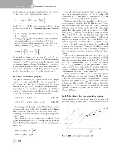
if: graph. Let h be a node in G, the state-times reachable
from h by a ð€ s; sÞ-bang lie on the grid, they are nodes
€ s only changes its value at times ks where k˛N; of G (Fig. 14.2-26). An edge between h and one of its
0 k Pt f =sR.
ks ks neighbours represents the corresponding ð€ s; sÞ-bang. A
Let€ s ðresp:€ s Þ be the minimum (resp. maximum)
min max sequence of edges between two nodes defines a ca-
acceleration allowed w.r.t. the state of A at time nonical trajectory. The time of such a canonical tra-
ks: € sðksÞ is chosen from D so as to be either null or as
ks ks jectory is trivially equal to s times the number of
close as possible to€ s and€ s . Thus we have:
min max edges in the trajectory. Therefore the shortest path
( " # " #) between two nodes (in term of number of edges) is
€ s ks € s ks
min
max
€ sðksÞ ˛ d ; 0; d the time-optimal canonical trajectory between these
d d nodes.
Let s ¼ðs i ; _ s i Þ be the initial state of A and g ¼ðs ; _ s Þ
f
f
As we will see later in this section, € s ks and € s ks are be its goal state. Without loss of generality it is assumed
min
max
computed so as to ensure that the acceleration constraint that the corresponding initial state-time s ) ¼ðs i ; _ s i ; 0Þ
(Equation 14.2.29) is respected along the trajectory until and the corresponding set of goal state-times
the next acceleration change. Note that such a trajectory G ¼fðs ; _ s ; ksÞwith k 0g are grid-points. Accord-
*
f
f
is very similar to the so-called ‘bang–bang’ trajectory of ingly searching for a time-optimal canonical trajectory
the control literature except that, in our case, the between s and g is equivalent to searching a shortest path
acceleration switches occur at regular time intervals. in G between the node s and a node in G .
)
)
From a practical point of view, the state-time graph
14.2.5.5.3 State-time graph G G is embedded in a compact region of ST. More pre-
cisely, the time component of the grid-points is upper
Let q be a state-time, i.e. a point of ST. It is a triple bounded by a certain value t max which can be viewed as
ðs; _ s; tÞ. It can equivalently be represented by a time-out. The number of grid-points is therefore
qðtÞ¼ðsðtÞ; _ sðtÞÞ.Let qðksÞ¼ðsðksÞ; _ sðksÞÞ be a state- finite and so is G. Accordingly the search for the time-
time of A and qððk þ 1ÞsÞ one of the state-times that A optimal canonical trajectory can be done in a finite
can reach by a canonical trajectory of duration amount of time.
s: qððk þ 1ÞsÞ is obtained by applying an acceleration € s ˛
D to A for the duration s. Accordingly we have:
14.2.5.5.4 Searching the state-time graph
_ sððK þ 1ÞsÞ¼ _ sðKsÞþ€ ss (14.2.32)
Search algorithm We use an A algorithm to search G
)
1 2 )
_ sððK þ 1ÞsÞ¼ sðKsÞþ _ sðKsÞs þ € ss (14.2.33) (Nilsson, 1980). Starting with s as the current node, we
2
By analogy with (Canny et al., 1988), the trajectory
between qðKsÞ and qððK þ 1ÞsÞ is called a ð€ s; sÞ-bang.
The state-time qððK þ 1ÞsÞ is reachable from qðKsÞ.
Obviously a canonical trajectory is made up of a sequence
of ð€ s; sÞ-bangs.
Let qðmsÞ; m K; be a state-time reachable from
qðKsÞ. Assuming that _ sðKsÞ is a multiple of sT, it can be
shown that the following relations hold for some integers
a 1 and a 2 :

1 2
sðmsÞ¼ sðKsÞþ a 1 ds
2
_ sðmsÞ¼ _ sðKsÞþ a 2 ds
Fig. 14.2-26 G, the graph embedded in ST .

462