Page 453 - Automotive Engineering Powertrain Chassis System and Vehicle Body

CHAP TER 1 4. 2 Decisional architecture

The final feasible accelerationrange istherefore given by by a pair ðs; _ sÞ ˛ j0; s max j j0; _ s max j where s max is the
the intersection of Equations 14.2.27 and 14.2.28: arc-length of S.
A state-time of A is defined by adding the time di-
q ffiffiffiffiffiffiffiffiffiffiffiffiffiffiffiffiffiffiffiffiffiffiffiffiffi
F min mension to a state hence it is represented by a triple
2 2
2 4
max ; m g k _ s € s
s
m ðs; _ s; tÞ ˛ j0; s max j j0; _ s max j j0; NÞ. The set of every
q ffiffiffiffiffiffiffiffiffiffiffiffiffiffiffiffiffiffiffiffiffiffiffiffiffi state-time is the state-time space of A; it is denoted by
F max
2 2
2 4
min ; m g k _ s ST.
s
m
A state-time is admissible if it does not violate the
no-collision and velocity constraints presented earlier.
14.2.5.4.2.5 Tangential velocity constraints Before defining an admissible state-time formally, let us
Velocity _ s must respect Equation 14.2.26. In addition, define T B’, the set of state-times which entail a collision
the argument under the square roots in Equation 14.2.28 between A and a moving obstacle. T B’ is simply derived
should be positive. When k s s0; _ s must respect the from T B:
following constraint:
0
r ffiffiffiffiffiffiffi r ffiffiffiffiffiffiffi T B ¼fðs; _ s; tÞjdi ˛ f1; .; bg; AðsÞXB i ðtÞsBg
mg mg
_ s (14.2.30)
jk s j jk s j Similarly we define T V’, the set of state-times which
violate the velocity constraint Equation 14.2.31. T V’ is
The final feasible velocity range is therefore given by simply derived from T V:
the intersection of Equations 14.2.26 and 14.2.30: r ffiffiffiffiffiffiffiffi
r ffiffiffiffiffiffiffi T V ¼ mg
0
mg ðs; _ s; tÞ 0 > _ s or _ s > min _ s max ; jK s j
0 _ s min _ s max ; (14.2.31)
jk s j
Accordingly a state-time q is admissible if and only if:
The latter constraint can be expressed as a set of
0
0
forbidden states, i.e. points of the s _ s plane. Let T V be q ˛ ST =ðT B W T V Þ
this set of states, it is defined as:
r ffiffiffiffiffiffiffi where E\F denotes the complement of F in E. The set of
mg every admissible state-time is the admissible state-time

T V ¼ ðs; _ sÞ 0 > _ s or _ s > min _ s max ;

jk s j space of A, it is denoted by AST and defined as:
0
0
AST ¼ ST =ðT B W T V Þ
14.2.5.4.3 Moving obstacles
2
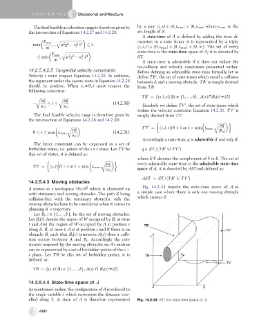
A moves in a workspace W˛R which is cluttered up Fig. 14.2-24 depicts the state-time space of A in
with stationary and moving obstacles. The path S being a simple case where there is only one moving obstacle
collision-free with the stationary obstacles, only the which crosses S.
moving obstacles have to be considered when it comes to
planning A’ s trajectory.
Let B i ; i ˛ f1; .; bg, be the set of moving obstacles.
Let B i (t) denote the region of W occupied by B i at time
t and A(s) the region of W occupied by A at position s
along S. If, at time t, A is at position s and if there is an
obstacle B i such that B i (t) intersects A(s) then a colli-
sion occurs between A and B i . Accordingly the con-
straints imposed by the moving obstacles on A’s motion
can be represented by a set of forbidden points of the s
t plane. Let T B be this set of forbidden points, it is
defined as:

T B ¼fðs; tÞjdi ˛ f1; .; bg; AðsÞ X B i ðtÞsBg

14.2.5.4.4 State-time space of A
As mentioned earlier, the configuration of A is reduced to
the single variable s which represents the distance trav-
elled along S. A state of A is therefore represented Fig. 14.2-24 ST ; the state-time space of A.

460