Page 454 - Automotive Engineering Powertrain Chassis System and Vehicle Body

Decisional architecture C HAPTER 14.2

in the previous section, was initially motivated by the
work described in Canny et al. (1988). For reasons which
will be discussed later in Section 14.2.5.5, we follow the
paradigm of near-time-optimization, i.e. instead of trying
to find out the exact time-optimal trajectory between an
initial and a final state, we compute an approximate
time-optimal solution by performing the search over
a restricted set of canonical trajectories. These canonical
trajectories are defined as having piecewise constant
acceleration€ s that can only change its value at given times
ks where s is a time-step and k some positive integer.
Besides € s is selected so as to be either minimum, null or
maximum. Under these assumptions, it is possible to
transform the problem of finding the time-optimal
canonical trajectory to finding the shortest path in a
directed graph G embedded in ST . The vertices G form
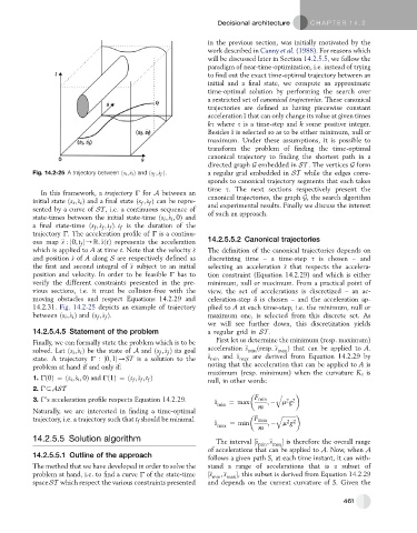
Fig. 14.2-25 A trajectory between ðs i ; _ s i Þ and ðs f ; _ s f Þ. a regular grid embedded in ST while the edges corre-
sponds to canonical trajectory segments that each takes
time s. The next sections respectively present the
In this framework, a trajectory G for A between an
initial state ðs i ; _ s i Þ and a final state ðs ; _ s Þ can be repre- canonical trajectories, the graph G, the search algorithm
f
f
sented by a curve of ST , i.e. a continuous sequence of and experimental results. Finally we discuss the interest
state-times between the initial state-time ðs i ; _ s i ; 0Þ and of such an approach.
a final state-time ðs ; _ s ; t Þ: t is the duration of the
f
f
f
f
trajectory G. The acceleration profile of G is a continu-
ous map € s : j0; t j/R: € sðtÞ represents the acceleration 14.2.5.5.2 Canonical trajectories
f
which is applied to A at time t. Note that the velocity _ s The definition of the canonical trajectories depends on
and position s ˙ of A along S are respectively defined as discretizing time – a time-step s is chosen – and
the first and second integral of € s subject to an initial selecting an acceleration € s that respects the accelera-
position and velocity. In order to be feasible G has to tion constraint (Equation 14.2.29) and which is either
verify the different constraints presented in the pre- minimum, null or maximum. From a practical point of
vious sections, i.e. it must be collision-free with the view, the set of accelerations is discretized – an ac-
moving obstacles and respect Equations 14.2.29 and celeration-step d is chosen – and the acceleration ap-
14.2.31. Fig. 14.2-25 depicts an example of trajectory plied to A at each time-step, i.e. the minimum, null or
between ðs i ; _ s i Þ and ðs ; _ s Þ. maximum one, is selected from this discrete set. As
f
f
we will see further down, this discretization yields
14.2.5.4.5 Statement of the problem a regular grid in ST .
Finally, we can formally state the problem which is to be First let us determine the minimum (resp. maximum)
solved. Let ðs i ; _ s i Þ be the state of A and ðs ; _ s Þ its goal acceleration € s min ðresp: € s max Þ that can be applied to A.
f
f
state. A trajectory G : j0; 1j/ST is a solution to the € s min and € s max are derived from Equation 14.2.29 by
problem at hand if and only if: noting that the acceleration that can be applied to A is
maximum (resp. minimum) when the curvature K S is
1. Gð0Þ¼ðs i ; _ s i ; 0Þ and Gð1Þ¼ðs f ; _ s f ; t f Þ
null, in other words:
2. G3AST
q ffiffiffiffiffiffiffiffiffiffi
3. G’s acceleration profile respects Equation 14.2.29. € s min ¼ max F min ; m g
2 2
Naturally, we are interested in finding a time-optimal m q ffiffiffiffiffiffiffiffiffiffi
trajectory, i.e. a trajectory such that t f should be minimal. F max
2 2
€ s max ¼ min m ; m g
14.2.5.5 Solution algorithm The interval ½€ s min ;€ s max Š is therefore the overall range
of accelerations that can be applied to A. Now, when A
14.2.5.5.1 Outline of the approach follows a given path S, at each time instant, it can with-
The method that we have developed in order to solve the stand a range of accelerations that is a subset of
problem at hand, i.e. to find a curve G of the state-time ½€ s min ;€ s max Š, this subset is derived from Equation 14.2.29
spaceST which respect the various constraints presented and depends on the current curvature of S. Given the

461