Page 715 - Automotive Engineering Powertrain Chassis System and Vehicle Body

CHAP TER 2 1. 1 Interior noise: Assessment and control

Differential equations The same rules apply to the well-known, second-order
differential equation characterising the motion of a mass
The input–output relations for networks that store on a spring with a viscous damper
energy (dynamic systems) are given by differential m€ x þ c_ x þ kx ¼ FðtÞ (A21.1.8)
equations.
Consider a linear, continuous-time system where: If two initial conditions are known, namely x(0)
The output is represented by y(t); and € xð0Þ, the value of x at some instant t later may be
The input is represented by x(t). found.
The two variables will be related by a differential equa-
tion of the form:
Appendix 21.1B: The convolution
n n 1
d y d y dy
a n þ a n 1 þ / þ a 1 þ a 0 y integral
dt n dt n 1 dt
m
d x
¼ b m þ / þ b 0 x (A21.1.1) Some aperiodic signals have unique properties and are
dt m
known as singularity functions because they are either
This equation is called a ‘linear differential equation of discontinuous or have discontinuous derivatives (Sinha,
order n’ and for most practical cases n P m. 1991). The simplest of these is the unit step function (as
d
It is convenient to replace dt by the operator ‘p’ illustrated in Fig. B21.1-1), given the symbol g(t)
resulting in the equation The unit impulse function or delta function d(t)is
defined as the function which after integration yields the
n
ða n p þ a n 1 p n 1 þ / þ a 1 p þ a 0 ÞyðtÞ unity step function, so (Sinha, 1991)
m
¼ðb m p þ / þ b 1 p þ b 0 ÞxðtÞ (A21.1.2) ð t
gðtÞ¼ dðsÞds (B21.1.1)
which may be written compactly as N
DðpÞyðtÞ¼ NðpÞxðtÞ (A21.1.3) Alternatively,
gðtÞ
where D( p) and N( p) are polynomials in the dðtÞ¼ (B21.1.2)
operator ‘p’ dt
The impulse function must satisfy:
n
DðpÞ¼ a n p þ a n 1 p n 1 þ / þ a 1 p þ a 0
(A21.1.4) dðtÞ¼ 0; for t not equal to zero (B21.1.3)
m
NðpÞ¼ b m p þ b m 1 p m 1 þ / þ b 1 p þ b 0 and
(A21.1.5) ð
N
dðtÞdt ¼ 1 (B21.1.4)
The operator ‘p’ does not satisfy the commutative
N
property
Therefore, the area under the impulse function is
pyðtÞsyðtÞp (A21.1.6) unity and it occurs over an infinitesimal interval around
t ¼ 0. So, as the period dt tends towards zero, the height
The system operator L( p) or transfer function is the of the impulse function approaches infinity.
ratio of the two polynomials D( p) and N( p)
Also,
NðpÞ
LðpÞ¼ (A21.1.7) ddðtÞ
DðpÞ ¼ N at t ¼ 0 and is zero elsewhere:
dt
Any dynamic system described by a differential
equation of order n can be solved uniquely only if at least
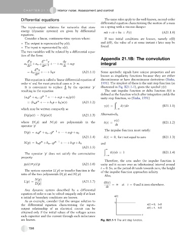
n initial or boundary conditions are known. x(t)
As an example, consider that the unique solution to
1
the differential equation characterising the input– x(t) = 0, t<0
output relationship of an electrical circuit can be x(t) = 1, t>0
obtained only if the initial values of the voltages across
each capacitor and the current through each inductance t
are known. Fig. B21.1-1 The unit step function.

726