Page 717 - Automotive Engineering Powertrain Chassis System and Vehicle Body

CHAP TER 2 1. 1 Interior noise: Assessment and control

F(x) is the probability of X taking a value up to and
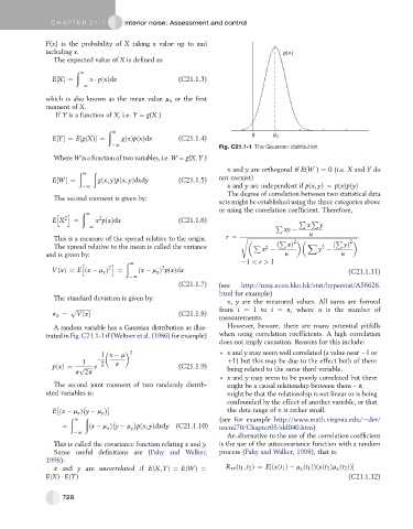
including x. p ( x )
The expected value of X is defined as:
ð
N
E½XŠ¼ x pðxÞdx (C21.1.3)
N
which is also known as the mean value m x or the first
moment of X.
If Y is a function of X, i.e. Y ¼ g(X )
ð
N
E½YŠ¼ E½gðXފ ¼ gðxÞpðxÞdx (C21.1.4) 0 x
N Fig. C21.1-1 The Gaussian distribution.

Where Wis a function of two variables, i.e. W ¼ g(X, Y )
ð ð x and y are orthogonal if E(W ) ¼ 0 (i.e. X and Y do
N
E½WŠ¼ gðx; yÞpðx; yÞdxdy (C21.1.5) not coexist)
N x and y are independent if pðx; yÞ¼ pðxÞpðyÞ
The degree of correlation between two statistical data
The second moment is given by:
sets might be established using the three categories above
h i ð N or using the correlation coefficient. Therefore,
2
E X 2 ¼ x pðxÞdx (C21.1.6) P P
N P x y
xy n
This is a measure of the spread relative to the origin. r ¼ s ffiffiffiffiffiffiffiffiffiffiffiffiffiffiffiffiffiffiffiffiffiffiffiffiffiffiffiffiffiffiffiffiffiffiffiffiffiffiffiffiffiffiffiffiffiffiffiffiffiffiffiffiffiffiffiffiffiffiffiffiffiffiffiffiffiffiffiffiffiffiffiffiffiffiffiffiffiffiffi
P
P

2
2
X
The spread relative to the mean is called the variance P x ð xÞ y ð yÞ
2
2
and is given by: n n
h i ð N 1 < r > 1
2
VðxÞ¼ E ðx m Þ 2 ¼ ðx m Þ pðxÞdx (C21.1.11)
x
x
N
(C21.1.7) (see http://max.econ.hku.hk/stat/hyperstat/A56626.
html for example)
The standard deviation is given by:
x, y are the measured values. All sums are formed
p ffiffiffiffiffiffiffiffiffiffi from i ¼ 1to i ¼ n, where n is the number of
s x ¼ VðxÞ (C21.1.8)
measurements.
A random variable has a Gaussian distribution as illus- However, beware, there are many potential pitfalls
trated in Fig. C21.1-1 if (Weltner et al. (1986) for example) when using correlation coefficients. A high correlation
does not imply causation. Reasons for this include:
2
1 x m x and y may seem well correlated (a value near 1or
1 2 þ1) but this may be due to the effect both of them
pðxÞ¼ p ffiffiffiffiffiffi e s (C21.1.9) being related to the same third variable.
s 2p
x and y may seem to be poorly correlated but there
The second joint moment of two randomly distrib- might be a causal relationship between them – it
uted variables is: might be that the relationship is not linear or is being
confounded by the effect of another variable, or that

E ðx m Þ y m y the data range of x is rather small.
x
ð ð
N (see for example http://www.math.virginia.edu/~der/
¼ ðx m Þ y m pðx; yÞdxdy (C21.1.10) useml70/Chapter05/sld040.htm)
x
y
N
An alternative to the use of the correlation coefficient
This is called the covariance function relating x and y. is the use of the autocovariance function with a random
Some useful definitions are (Fahy and Walker, process (Fahy and Walker, 1998), that is:
1998):
x and y are uncorrelated if EðX; YÞ¼ EðWÞ¼ R xx ðt 1 ; t 2 Þ¼ E½ðxðt 1 Þ m ðt 1 ÞÞðxðt 2 Þm ðt 2 Þފ
x
x
EðXÞ EðYÞ (C21.1.12)
728