Page 716 - Automotive Engineering Powertrain Chassis System and Vehicle Body

Interior noise: Assessment and control C HAPTER 21.1

Consider a unit impulse that occurs at time t ¼ s as x(t)
illustrated in Fig. B21.1-2
Remember that the definition of the unit impulse
requires it to occur at time t ¼ 0. Therefore, shift the
time axis in the Fig. B21.1-2 by the amount required
for t ¼ s ¼ 0. Therefore, the unit impulse occurring at
time t ¼ s is assigned with the symbol d(t s). –Δ 0 +Δ t
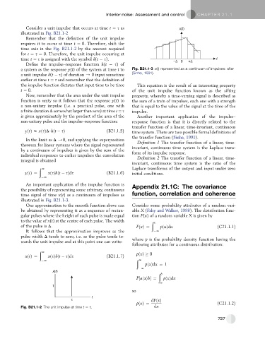
Define the impulse–response function h(t s)of
a system as the response y(t) of the system at time t to Fig. B21.1-3 x(t) represented as a continuum of impulses: after
a unit impulse d(t s) of duration / 0 input sometime (Sinha, 1991).
earlier at time t ¼ s and remember that the definition of
the impulse function dictates that input time to be time This equation is the result of an interesting property
t ¼ 0. of the unit impulse function known as the sifting
Now, remember that the area under the unit impulse property, whereby a time-varying signal is described as
function is unity so it follows that the response y(t)to the sum of a train of impulses, each one with a strength
a non-unitary impulse (i.e. a practical pulse, one with that is equal to the value of the signal at the time of the
a finite duration D somewhat larger than zero) at time t ¼ s impulse.
is given approximately by the product of the area of the Another important application of the impulse–
non-unitary pulse and the impulse–response function: response function is that it is directly related to the
transfer function of a linear, time-invariant, continuous
yðtÞ z xðsÞD$hðt sÞ (B21.1.5) time system. There are two possible formal definitions of
the transfer function (Sinha, 1991).
In the limit as D /0, and applying the superposition
Definition 1 The transfer function of a linear, time-
theorem for linear systems where the signal represented invariant, continuous time system is the Laplace trans-
by a continuum of impulses is given by the sum of the form of its impulse response.
individual responses to earlier impulses the convolution Definition 2 The transfer function of a linear, time-
integral is obtained
invariant, continuous time system is the ratio of the
ð N Laplace transforms of the output and input under zero
yðtÞ¼ xðsÞhðt sÞds (B21.1.6) initial conditions.
N
An important application of the impulse function is Appendix 21.1C: The covariance
the possibility of representing some arbitrary, continuous
time signal of time x(t) as a continuum of impulses as function, correlation and coherence
illustrated in Fig. B21.1-3.
One approximation to the smooth function above can Consider some probability attributes of a random vari-
be obtained by representing it as a sequence of rectan- able X (Fahy and Walker, 1998). The distribution func-
gular pulses where the height of each pulse is made equal tion F(x) of a random variable X is given by
to the value of x(t) at the centre of each pulse. The width ð x
of the pulse is D. FðxÞ¼ pðuÞdu (C21.1.1)
It follows that the approximation improves as the N
pulse width D tends to zero, i.e. as the pulse tends to- where p is the probability density function having the
wards the unit impulse and at this point one can write:
following attributes for a continuous distribution:
ð N
xðtÞ¼ xðsÞdðt sÞds (B21.1.7) pðxÞ 0
N ð N
pðxÞdx ¼ 1
N
x(t) ð
b
P½ahxibŠ ¼ pðxÞdx
a
1
so

τ t dFðxÞ
pðxÞ¼ (C21.1.2)
Fig. B21.1-2 The unit impulse at time t ¼ s. dx

727