Page 137 - Autonomous Mobile Robots

120 Autonomous Mobile Robots

^ x ^
x k|k-1 + k|k
Dynamic motion
+
dx ^ k|k
Measurement Kalman filter
prediction
Ephemeris Predicted measurements
–
Measurement residuals
GPS
Measurements
+
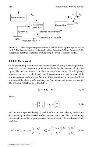
FIGURE 3.1 Block diagram representation for a GPS-only navigation system solved
via KF. The dynamic motion prediction by either Equation (3.21) or Equation (3.38)
extrapolates from the present state estimate using the assumed dynamic model.

3.3.3.1 Clock model

Global positioning system receivers use oscillators with very stable frequencies.
Integration of this frequency provides the basis for the receiver clock time
signal. The error between the oscillator frequency and its specified frequency
represents the receiver clock drift rate. It is common to model the clock drift
rate as a random walk process. We scale these quantities by the speed of light
to represent the clock bias b u and drift rate f u in meters and meters per second.
T
The dynamic model for x c =[b u , f u ] is

˙ x c = F c x c + w c (3.53)

where

0 1 ω b
F c = , w c = , (3.54)
0 0 ω f
and the power spectral density S b and S f of the process noise ω b and ω f are
determined by the characteristics of the receiver clock [20]. The corresponding
state transition matrix and process noise covariance matrix for the discrete clock
model are:

 3 2 
t t

1 t S b t + S f 3 S f 2
c c c
= (t k , t k+1 ) = , Q =   (3.55)
k 0 1 k t 2
S f 2 S f t

© 2006 by Taylor & Francis Group, LLC

FRANKL: “dk6033_c003” — 2006/3/31 — 16:42 — page 120 — #22