Page 140 - Autonomous Mobile Robots

Data Fusion via Kalman Filter 123

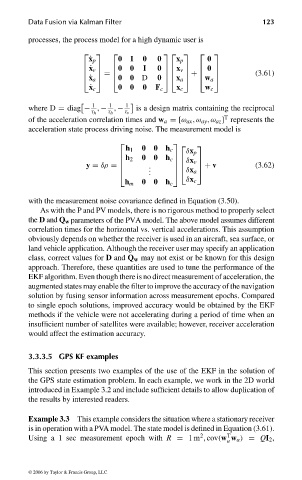
processes, the process model for a high dynamic user is

       
0 I 0 0 0
˙ x p x p
0 0 I 0 0
˙ x v x v
       
  =     +   (3.61)
 ˙ x a   0 0 D 0   x a   w a 
˙ x c 0 0 0 F c x c w c
1 1 1

where D = diag − , − , − is a design matrix containing the reciprocal
τ h τ h τ v
T
of the acceleration correlation times and w a =[ω ax , ω ay , ω az ] represents the
acceleration state process driving noise. The measurement model is
   
h 1 0 0 h c
δx p
 h 2 0 0 
 δx v 
h c 
.   
 + v (3.62)
.  δx a 
y = δρ = 

 .
h m 0 0 h c δx c
with the measurement noise covariance defined in Equation (3.50).
As with the P and PV models, there is no rigorous method to properly select
the D and Q w parameters of the PVA model. The above model assumes different
correlation times for the horizontal vs. vertical accelerations. This assumption
obviously depends on whether the receiver is used in an aircraft, sea surface, or
land vehicle application. Although the receiver user may specify an application
class, correct values for D and Q w may not exist or be known for this design
approach. Therefore, these quantities are used to tune the performance of the
EKF algorithm. Even though there is no direct measurement of acceleration, the
augmented states may enable the filter to improve the accuracy of the navigation
solution by fusing sensor information across measurement epochs. Compared
to single epoch solutions, improved accuracy would be obtained by the EKF
methods if the vehicle were not accelerating during a period of time when an
insufficient number of satellites were available; however, receiver acceleration
would affect the estimation accuracy.

3.3.3.5 GPS KF examples
This section presents two examples of the use of the EKF in the solution of
the GPS state estimation problem. In each example, we work in the 2D world
introduced in Example 3.2 and include sufficient details to allow duplication of
the results by interested readers.

Example 3.3 This example considers the situation where a stationary receiver
is in operation with a PVA model. The state model is defined in Equation (3.61).
2
T
Using a 1 sec measurement epoch with R = 1m ,cov(w w a ) = QI 2 ,
a

© 2006 by Taylor & Francis Group, LLC

FRANKL: “dk6033_c003” — 2006/3/31 — 16:42 — page 123 — #25