
Page 143 - Autonomous Mobile Robots
P. 143
126 Autonomous Mobile Robots
(b) Trajectory vs. EKF estimated
15
10
y (m) 5
0 Q=10
– 5
0 200 400 600 800
15
10
y (m) 5
0 Q=1
– 5
0 200 400 600 800
15
10
y (m) 5
0 Q=0.1
– 5
0 200 400 600 800
15
10
y (m) 5
0 Q=0.01
– 5
0 200 400 600 800
15
10
y (m) 5
0 Q=0.001
– 5
0 200 400 600 800
Position, x (m)
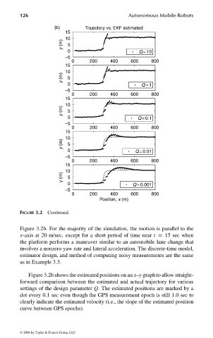
FIGURE 3.2 Continued.
Figure 3.2b. For the majority of the simulation, the motion is parallel to the
x-axis at 20 m/sec, except for a short period of time near t = 15 sec when
the platform performs a maneuver similar to an automobile lane change that
involves a nonzero yaw rate and lateral acceleration. The discrete-time model,
estimator design, and method of computing noisy measurements are the same
as in Example 3.3.
Figure 3.2b shows the estimated positions on an x–y graph to allow straight-
forward comparison between the estimated and actual trajectory for various
settings of the design parameter Q. The estimated positions are marked by a
dot every 0.1 sec even though the GPS measurement epoch is still 1.0 sec to
clearly indicate the estimated velocity (i.e., the slope of the estimated position
curve between GPS epochs).
© 2006 by Taylor & Francis Group, LLC
FRANKL: “dk6033_c003” — 2006/3/31 — 16:42 — page 126 — #28