Page 138 - Autonomous Mobile Robots

Data Fusion via Kalman Filter 121

where t = t k+1 − t k . This clock model will be included as a portion of the
model in each of the following sections.

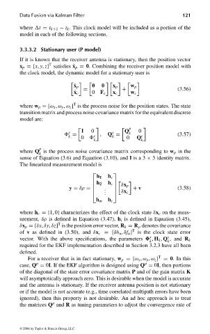
3.3.3.2 Stationary user (P model)
If it is known that the receiver antenna is stationary, then the position vector
T
x p =[x, y, z] satisfies ˙ x p = 0. Combining the receiver position model with
the clock model, the dynamic model for a stationary user is

˙ x p 0 0 x p w p
= + (3.56)
˙ x c 0 F c x c w c
T
where w p =[ω x , ω y , ω z ] is the process noise for the position states. The state
transition matrix and process noise covariance matrix for the equivalent discrete
model are:

p
I 0 Q 0
s s k
= , Q = (3.57)
k 0 c k 0 Q c
k k
p
where Q is the process noise covariance matrix corresponding to w p in the
k
sense of Equation (3.6) and Equation (3.10), and I isa3 × 3 identity matrix.
The linearized measurement model is
 
h 1 h c

h 2 h c
 
 δx p

. + v (3.58)
.  δx c
y = δρ =  
 .
h m h c
where h c =[1, 0] characterizes the effect of the clock state δx c on the meas-
urement, δρ is defined in Equation (3.47), h i is defined in Equation (3.45),
T
δx p =[δx, δy, δz] is the position error vector, R k = R ρ denotes the covariance
T
of v as defined in (3.50), and δx c =[δb u , δf u ] is the clock state error
s s
vector. With the above specifications, the parameters , H k , Q , and R k
k k
required for the EKF implementation described in Section 3.2.3 have all been
defined.
T
For a receiver that is in fact stationary, w p =[ω x , ω y , ω z ] = 0. In this
p
p
case, Q = 0I. If the EKF algorithm is designed using Q = 0I, then portions
of the diagonal of the state error covariance matrix P and of the gain matrix K
will asymptotically approach zero. This is desirable when the model is accurate
and the antenna is stationary. If the receiver antenna position is not stationary
or if the model is not accurate (e.g., time correlated multipath errors have been
ignored), then this property is not desirable. An ad hoc approach is to treat
p
the matrices Q and R as tuning parameters to adjust the convergence rate of
© 2006 by Taylor & Francis Group, LLC

FRANKL: “dk6033_c003” — 2006/3/31 — 16:42 — page 121 — #23