Page 139 - Autonomous Mobile Robots
P. 139

122                                    Autonomous Mobile Robots

                                the filter. However, a far better approach is to develop a more appropriate system
                                model.


                                3.3.3.3 Low dynamic user (PV Model)
                                For a receiver in a “low dynamic environment” it may be reasonable to assume
                                that the velocity vector is a random walk process. In this case, an eight
                                state model is appropriate with the acceleration vector modeled as white noise.
                                The state vector includes the position state x p , receiver clock state x c , and
                                                        T
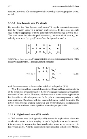
                                velocity state x v =[v x , v y , v z ] ; therefore, the dynamic model is
                                                                       
                                                         0  I  0            0
                                                  ˙ x p             x p
                                                 ˙ x v = 0  0  0  x v + w v       (3.59)
                                                       
                                                 
                                                                          
                                                                   
                                                                              
                                                         0  0
                                                  ˙ x c        F c  x c    w c
                                                      T
                                where w v =[ω vx , ω vy , ω vz ] represents the process noise representation of the
                                unknown acceleration. The measurement model is
                                                                   
                                                           h 1  0
                                                                          
                                                                  h c 
                                                          h   0     δx p
                                                          2      h c
                                                                     
                                                                          
                                                 y = δρ =     .      δx v + v         (3.60)
                                                              .    
                                                              .    
                                                                       δx c
                                                               0
                                                          h m     h c
                                with the measurement noise covariance defined in Equation (3.50).
                                   Wewillnotprovideanin-depthdiscussionofthismodelhere, asthemajority
                                of the comments about the model of the following section are also applicable to
                                the model of this section. However, it is important to note that few applications
                                involve white acceleration processes. In fact, the acceleration process is rarely
                                even stationary. Therefore, with this assumed dynamic model, the matrix Q w
                                is best considered as a tuning parameter and proper stochastic interpretations
                                of the various variables in the algorithm are no longer applicable.

                                3.3.3.4 High dynamic user (PVA model)

                                A GPS receiver may (and typically will) operate in applications where the
                                acceleration vector is time varying. In such “high dynamic environments,”
                                                                                           T
                                it is necessary to augment the three acceleration states x a =[a x , a y , a z ] to
                                the system model. With the acceleration states modeled as first-order Markov


                                 © 2006 by Taylor & Francis Group, LLC


                                FRANKL: “dk6033_c003” — 2006/3/31 — 16:42 — page 122 — #24
   134   135   136   137   138   139   140   141   142   143   144