Page 141 - Autonomous Mobile Robots

124 Autonomous Mobile Robots

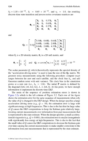
S b = 1.10 × 10 −10 , S f = 0.65 × 10 −10 , and τ h = 1.0, the resulting
discrete-time state transition and process noise covariance matrices are

 
I 2 I 2 0.37I 2 0 2
0 2 I 2 0.63I 2 0 2
 
k =  
 0 2 0 2 0.37I 2 0 2 
0 2 0 2 0 2 c
and

   
0.30I 2 0.68I 2 0.64I 2 0 2
  0.68I 2 1.68I 2 2.00I 2  0 2 
Q k =  0.1Q 
 0.64I 2 2.00I 2 4.33I 2 0 2 
0 2 0 2 0 2 Q c
where I 2 is a 2D identity matrix, 0 2 is a 2D null matrix, and

1 1 T 1.32 0.32 −10
c = and Q c = cov(w w c ) = × 10
c
0 1 0.32 0.65
The scalar parameter Q, which theoretically represents the spectral density of
the “acceleration driving noise,” is used to tune the size of the Q k matrix. We
generate noisy measurements using the following procedure: compute exact
ranges between the user and each satellite, add the clock bias b u , and add
Gaussian random noise with unit variance. The clock bias in the simulation
grows at a unit rate (i.e., b u = 1.0t). The initial P matrix is defined by
the diagonal [1e6, 1e6, 1e2, 1e2, .1, .1, 1e6, 1]. At this point, we have enough
information to implement the discrete-time EKF.
The norm of the sequence of position estimation errors is shown in
Figure 3.2a which is the left column of Figure 3.2. Each row of the figure
shows the estimation error for the same sequence of measurements when only
the value of Q is changed in the EKF design. When the design specifies a large
acceleration driving noise (e.g., Q = 10), the estimation error is large with
significant energy at high frequencies. This is due to the fact that the large value
of Q causes the EKF computations to keep the Kalman gain relatively large,
favoring current measurements over information from past measurements that
is represented by the state estimate. When the design specifies a small accelera-
tion driving noise (e.g., Q = 0.001), the estimation error is smaller in magnitude
with significantly less energy at high frequencies. This is due to the fact that
the small value of Q causes the EKF computations to decrease the Kalman gain
over time causing the current measurements to make smaller corrections to the
information from past measurements that is represented by the state estimate.

© 2006 by Taylor & Francis Group, LLC

FRANKL: “dk6033_c003” — 2006/3/31 — 16:42 — page 124 — #26