Page 347 - Autonomous Mobile Robots

Map Building and SLAM Algorithms 337

(a) 15
10

5
0 x y
–5
–10
–15 x y x y
–20

–25
–20 –10 0 10 20 30 40
(b) 15
10
5
0 x y

–5
–10
x y x y
–15
–20

–25
–20 –10 0 10 20 30 40
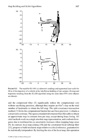
FIGURE 9.1 The need for SLAM: (a) odometric readings and segmented laser walls for
40 m of the trajectory of a vehicle at the Ada Byron building of our campus; (b) map and
trajectory resulting from the SLAM algorithm using the same data (95% error ellipses
are drawn).

and the compressed filter [3] significantly reduce the computational cost
2
without sacrificing precision, although they require an O(n ) step on the total
number of landmarks to obtain the full map. The split covariance intersection
method [7] limits the computational burden but sacrifices precision: it obtains a
conservativeestimate. Thesparseextendedinformationfilter[8]isabletoobtain
an approximate map in constant time per step, except during loop closing. All
cited methods work on a single absolute map representation, and confront diver-
gence due to nonlinearities as uncertainty increases when mapping large areas
[9]. In contrast, local map joining [10] and the constrained local submap filter
[11], propose to build stochastic maps relative to a local reference, guaranteed to
be statistically independent. By limiting the size of the local map, this operation

© 2006 by Taylor & Francis Group, LLC

FRANKL: “dk6033_c009” — 2006/3/31 — 16:43 — page 337 — #7