Page 352 - Autonomous Mobile Robots

342 Autonomous Mobile Robots

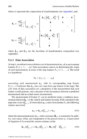
where ⊕ represents the composition of transformations (see Appendix), and:

 
J 1⊕ ˆ x B , ˆ x R k−1 0 ··· 0
R k−1 R k
 

∂x B  . 
 0 I . . 
k|k−1
F k = =  
∂x B R k−1  . . . . 
k−1 (ˆ x B , ˆ x )  . . 
k−1 R k  
0 ··· I

 
J 2⊕ ˆ x B , ˆ x R k−1

R k−1 R k
∂x B  
k|k−1  0 
G k = =  . 
∂x R k−1  . 
R k B R k−1  . 
(ˆ x , ˆ x )
k−1 R k
0
where J 1⊕ and J 2⊕ are the Jacobians of transformation composition (see
Appendix).
9.2.3 Data Association
At step k, an onboard sensor obtains a set of measurements z k,i of m environment
features E i (i = 1, ... , m). Data association consists in determining the origin
of each measurement, in terms of the map features F j , j = 1, ... , n. The result
is a hypothesis:
H k =[j 1 j 2 ··· j m ]
associating each measurement z k,i with its corresponding map feature
(j i = 0 indicates that z k,i does not come from any feature in the map). The
F j i
core tools of data association are a prediction of the measurement that each
feature would generate, and a measure of the discrepancy between a predicted
measurement and an actual sensor measurement.
The measurement of feature F j can be predicted using a nonlinear meas-
urement function h k, j of the vehicle and feature location, both contained in the
map state vector x B . If observation z k,i comes from feature F j , the following
k|k−1
relation must hold:
z k,i = h k, j (x B ) + w k,i (9.5)
k|k−1
where the measurement noise w k,i , with covariance R k,i , is assumed to be addit-
ive, zero-mean, white, and independent of the process noise v k . Linearization
of Equation (9.5) around the current estimate yields:

B
h k, j (x B ) h k, j (ˆ x B ) + H k, j (x − ˆ x B ) (9.6)
k|k−1 k|k−1 k k|k−1

© 2006 by Taylor & Francis Group, LLC

FRANKL: “dk6033_c009” — 2006/3/31 — 16:43 — page 342 — #12