Page 354 - Autonomous Mobile Robots

344 Autonomous Mobile Robots

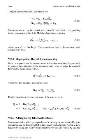
The joint innovation and its covariance are:

(ˆ x B )
k|k−1
ν H k = z k − h H k
(9.12)
B
P H T
S H k = H H k k + R H k
H k
Measurements z k can be considered compatible with their corresponding
features according to H k if the Mahalanobis distance satisfies:
D 2 = ν T S −1 ν H k <χ 2 (9.13)
H k H k H k d,1−α
). This consistency test is denominated joint
where now d = dim(h H k
compatibility (JC).

9.2.4 Map Update: The EKF Estimation Step
Once correspondences for measurements z k have been decided, they are used
to improve the estimation of the stochastic state vector by using the standard
EKF update equations as follows:

B
ˆ x = ˆ x B ν (9.14)
k k|k−1 + K H k H k
is obtained from:
where the filter gain K H k

= P B H T S −1 (9.15)
k|k−1 H k H k
K H k
Finally, the estimated error covariance of the state vector is:

B B
k k|k−1
P = (I − K H k H H k )P
)P B T K T (9.16)
k|k−1 H k
= (I − K H k H H k (I − K H k H H k ) + K H k R H k
9.2.5 Adding Newly Observed Features

Measurements for which correspondences in the map cannot be found by data
association can be directly added to the current stochastic state vector as new
features by using the relative transformation between the vehicle R k and the

© 2006 by Taylor & Francis Group, LLC

FRANKL: “dk6033_c009” — 2006/3/31 — 16:43 — page 344 — #14