Page 355 - Autonomous Mobile Robots

Map Building and SLAM Algorithms 345

B
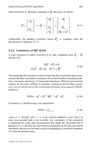
observed feature E. Therefore, updating of x takes place as follows:
k
 B   B 
x x
 B  R k R k
x
R k  .   . . 
 .   . 
B  .  B
.
x =  .   .    (9.17)
k ⇒ x + =  B  =  B 
k
  x   x 
x B  F n,k  F n,k 
F n,k B B R k
x x ⊕ x
E k R k E
B
Additionally, the updated covariance matrix P + is computed using the
k
linearization of Equation (9.17).
9.2.6 Consistency of EKF–SLAM
B
A state estimator is called consistent if its state estimation error x − ˆ x B
k k
satisfies [29]:
B
B
E[x − ˆ x ]= 0
k k
(9.18)
B
B T
B
B
E[(x − ˆ x )(x − ˆ x ) ]≤ P k B
k
k
k
k
This means that the estimator is unbiased and that the actual mean square error
matches the filter-calculated covariances. Given that SLAM is a nonlinear prob-
lem, consistency checking is of paramount importance. When the ground truth
solution for the state variables is available, a statistical test for filter consist-
ency can be carried out on the normalized estimation error squared (NEES),
defined as:
B
B
B −1
B T
B
NEES = (x − ˆ x ) (P ) (x − ˆ x ) (9.19)
k
k
k
k
k
Consistency is checked using a chi-squared test:
2
NEES ≤ χ d,1−α (9.20)
B
where d = dim(x ) and 1 − α is the desired confidence level. Since in
k
most cases ground truth is not available, the consistency of the estimation
is maintained by using only measurements that satisfy the innovation test of
Equation (9.13). Because the innovation term depends on the data association
hypothesis, this process becomes critical in maintaining a consistent estimation
[9] of the environment map.
© 2006 by Taylor & Francis Group, LLC

FRANKL: “dk6033_c009” — 2006/3/31 — 16:43 — page 345 — #15