Page 351 - Autonomous Mobile Robots

Map Building and SLAM Algorithms 341

assignment of an initial level of uncertainty to the estimated vehicle location.
In the theoretical linear case [26], the vehicle uncertainty should always remain
above this initial level. In practice, due to linearizations, when a nonzero initial
uncertainty is used, the estimated vehicle uncertainty rapidly drops below its
initial value, making the estimation inconsistent after very few EKF update
steps [9].
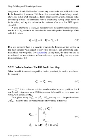
A good alternative is to use, as base reference, the current vehicle location,
that is, B = R 0 , and thus we initialize the map with perfect knowledge of the
vehicle location:

B
B
ˆ x = ˆ x B = 0; P = P B = 0 (9.2)
0 R 0 0 R 0
If at any moment there is a need to compute the location of the vehicle or
the map features with respect to any other reference, the appropriate trans-
formations can be applied (see Appendix). At any time, the map can also be
transformed to use a feature as base reference, again using the appropriate
transformations [10].

9.2.2 Vehicle Motion: The EKF Prediction Step
When the vehicle moves from position k −1 to position k, its motion is estimated
by odometry:

x R k−1 = ˆ x R k−1 + v k (9.3)
R k R k

where ˆ x R k−1 is the estimated relative transformation between positions k − 1
R k
and k, and v k (process noise [27]) is assumed to be additive, zero-mean, and
white, with covariance Q k .
B B B
Thus, given a map M = (ˆ x , P ) at step k − 1, the predicted map
k−1 k−1 k−1
B
M at step k after the vehicle motion is obtained as follows:
k|k−1
 B R k−1 
ˆ x ⊕ ˆ x
R k−1 R k
 
 ˆ x B 
ˆ x B  F 1,k−1 
k|k−1 =  . 
 .  (9.4)
 . 
ˆ x B
F m,k−1
T
P B F k P B F + G k Q k G T
k|k−1 k−1 k k

© 2006 by Taylor & Francis Group, LLC

FRANKL: “dk6033_c009” — 2006/3/31 — 16:43 — page 341 — #11