Page 349 - Autonomous Mobile Robots

Map Building and SLAM Algorithms 339

successful SLAM schemes must incorporate: (1) Data association techniques,
to relate sensor measurements with features already in the map, as well as
to decide those that are spurious or correspond to environment features not
previously observed, and (2) Loop closing and relocation techniques, that allow
determination of the vehicle location and correct the map when the vehicle
uncertainty increases significantly during exploration, or when there is no prior
information on the vehicle location. Finally, we point out the main open prob-
lem of the current state-of-art SLAM approaches: mapping large-scale areas.
Relevant shortcomings of this problem are, on the one hand, the computational
burden, which limits the applicability of the EKF-based SLAM in large-scale
real time applications and, on the other hand, the use of linearized solutions
which jeopardizes the consistency of the estimation process. We point out prom-
ising directions of research using nonlinear estimation techniques, and mapping
schemes for multivehicle SLAM.

9.2 SLAM USING THE EXTENDED KALMAN FILTER
In feature-based approaches to SLAM, the environment is modeled as a set
of geometric features, such as straight line segments corresponding to doors or
window frames, planes corresponding to walls, or distinguishable points in out-
door environments. The process of segmentation of raw sensor data to obtain
featureparametersdependsonthesensorandthefeaturetype. Inindoorenviron-
ments, laser readings can be used to obtain straight wall segments [21,22], or in
outdoor environments to obtain two-dimensional (2D) points corresponding to
trees and street lamps [3]. Sonar measurement environments can be segmented
into corners and walls [10]. Monocular images can provide information about
vertical lines [23] or interest points [24]. Even measurements from different
sensors can be fused to obtain feature information [25].
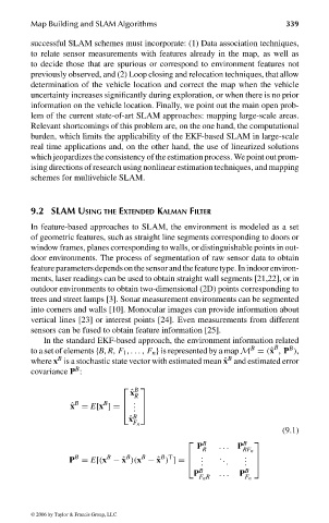
In the standard EKF-based approach, the environment information related
B
B
B
to a set of elements {B, R, F 1 , ... , F n } is represented by a map M = (ˆ x , P ),
B
B
where x is a stochastic state vector with estimated mean ˆ x and estimated error
B
covariance P :
 B 
ˆ x
R
B B  . 
.
ˆ x = E[x ]=  . 
ˆ x B
F n
(9.1)
P ... P
 B B 
R RF n
 .
B
B
B
B
B T
P = E[(x − ˆ x )(x − ˆ x ) ]=  . . . . . . 
.
. 
P B ... P B
F n R F n
© 2006 by Taylor & Francis Group, LLC
FRANKL: “dk6033_c009” — 2006/3/31 — 16:43 — page 339 — #9