Page 94 - Basics of Fluid Mechanics and Introduction to Computational Fluid Dynamics

Dynamics of Inviscid Fluids 79

oO é
0.57

OF

-1 oa 1 »
x

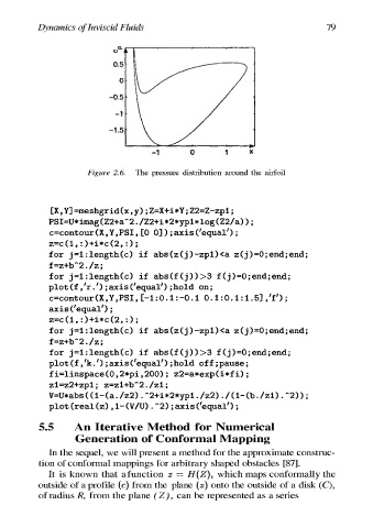
Figure 2.6. The pressure distribution around the airfoil

y)
;
(X,Y]=meshgrid(x, Z2=Z-zp1;
;Z=X+i*Y
PSI=U*imag(Z2+a~2./Z2+i*2*yp1*log(Z2/a))
;
;
c=contour(X,Y,PSI, [0 0]) ;axis(‘equal’)
z=c(1,:)+i*c(2,:);
for j=i:length(c) if abs(z(j)-zpi)<a z(j)=0;end;end;
f=z+b°2./z;
for j=i:length(c) if abs(f£(j))>3 £(j)=0;end;end;
plot (f,/r.') ;axis (‘equal’) ;hold on;
c=contour(X,Y,PSI, [-1:0.1:-0.1 0.1:0.1:1.5],’£");
axis (‘equal’) ;

z=c(1,:)+i*c(2,:);
for j=1:length(c) if abs(z(j)-zp1)<a z(j)=0;end;end;
f=z+b°2./z;
for j=1:length(c) if abs(f(j))>3 £(j)=0;end;end;
;hold
plot (f£,’k.’) ;axis(‘equal’)
off;pause;
fi=linspace(0,2*pi,200); z2=a*exp(i*fi)
;
zi=z2+zp1; z=zit+b°2./z1;
./(1-(b./z1)
.72));
V=U*abs ((1-(a./z2) .~2+i*2*yp1./z2)
;
plot (real (z) ,1-(V/U) .*2) ;axis(‘equal’)
5.5 An Iterative Method for Numerical
Generation of Conformal Mapping

In the sequel, we will present a method for the approximate construc-
tion of conformal mappings for arbitrary shaped obstacles [87].
It is known that afunction z = H(Z), which maps conformally the
outside of a profile (c) from the plane (z) onto the outside of a disk (C),

of radius R, from the plane (Z), can be represented as a series