Page 88 - Becoming Metric Wise

78 Becoming Metric-Wise

Figure 4.6 An empirical cumulative distribution.

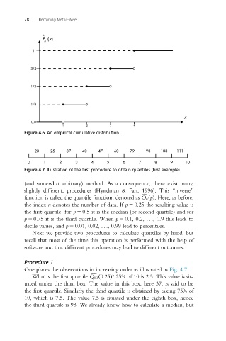
Figure 4.7 Illustration of the first procedure to obtain quantiles (first example).

(and somewhat arbitrary) method. As a consequence, there exist many,
slightly different, procedures (Hyndman & Fan, 1996). This “inverse”
function is called the quantile function, denoted as Q n ðpÞ. Here, as before,
c
the index n denotes the number of data. If p 5 0.25 the resulting value is
the first quartile: for p 5 0.5 it is the median (or second quartile) and for
p 5 0.75 it is the third quartile. When p 5 0.1, 0.2, .. ., 0.9 this leads to
decile values, and p 5 0.01, 0.02, .. ., 0.99 lead to percentiles.
Next we provide two procedures to calculate quantiles by hand, but
recall that most of the time this operation is performed with the help of
software and that different procedures may lead to different outcomes.

Procedure 1
One places the observations in increasing order as illustrated in Fig. 4.7.
What is the first quartile Q 10 ð0:25Þ? 25% of 10 is 2.5. This value is sit-
d
uated under the third box. The value in this box, here 37, is said to be
the first quartile. Similarly the third quartile is obtained by taking 75% of
10, which is 7.5. The value 7.5 is situated under the eighth box, hence
the third quartile is 98. We already know how to calculate a median, but