Page 501 - Biaxial Multiaxial Fatigue and Fracture

Geometry Variation and Life Estimates of Biaxial Fatigue Specimens 485

plotted on the Sines Z-O ellipse using results from different combinations of bending and
torsion tests.
Shatil and Smith [6, 191 developed a subsurface strain based model that was mainly used to
overcome conservative predictions of notched components when using biaxial fatigue results
obtained from testing of thin walled specimens [4]. Past experimental results were used to
examine the high-strain model [6] and it appeared to improve the conservative predictions
obtained by using thin walled biaxial data and surface values of multiaxial strain parameter
based on the critical plane approach [15].
The main advantage of the high-strain model was that it was not restricted to any particular
multiaxial fatigue parameter. However, the model’s physical interpretation was not fully
explained and, in particular, the subsurface critical distance was chosen somewhat arbitrarily,
considered to be lmm since it was the thickness of the thin walled specimens. This model is
further used in this work, and its main numerical development is given below.
The model is based on the folIowing assumptions:
A critical high-strain path was used through a net section. The critical path is evaluated up
to a depth of lmm distance from the surface of the notch net section. This distance was
chosen since it was the wall thickness of the hollow specimen.
The subsurface multiaxial strain along a critical path was divided into equal increments,
typically between 5 to 10 increments, and the life corresponding to the average strain from
each increment was obtained.
Considering that fatigue damage initiates on the surface, the contribution of damage from
each increment of strain under the surface was assumed to decrease with the distance from
the surface.
A linear accumulation of subsurface damage was used along the critical path.
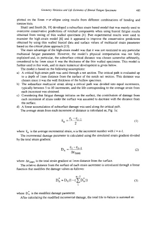
The average strain from each increment of distance is calculated as, Fig. la:

where En is the average incremental strain, n is the increment number with i = n-1.
The incremental damage parameter is calculated using the simulated strain gradient divided
by the total strain gradient:

where A&lm is the total strain gradient at lmm distance from the surface.
The relative distance from the surface of each strain increment is introduced through a linear
function that modifies the damage values as follows:

where D*, is the modified damage parameter.
After calculating the modified incremental damage, the total life to failure is summed as: