Page 71 - Big Data Analytics for Intelligent Healthcare Management

64 CHAPTER 4 TRANSFER LEARNING AND SUPERVISED CLASSIFIER

X2 Class 1

Class 2

Optimal hyperplane

Maximum margin

X1
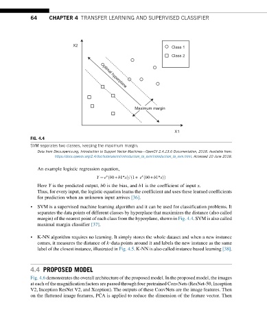
FIG. 4.4
SVM separates two classes, keeping the maximum margin.
Data from Docs.opencv.org, Introduction to Support Vector Machines—OpenCV 2.4.13.6 Documentation, 2018. Available from:
https://docs.opencv.org/2.4/doc/tutorials/ml/introduction_to_svm/introduction_to_svm.html, Accessed 10 June 2018.

An example logistic regression equation,
x x
Y ¼ e b0+ b1∗xÞ= 1+ e b0+ b1∗xÞÞ
ð
ð
ð
Here Y is the predicted output, b0 is the bias, and b1 is the coefficient of input x.
Thus, for every input, the logistic equation learns the coefficient and uses these learned coefficients
for prediction when an unknown input arrives [36].
• SVM is a supervised machine learning algorithm and it can be used for classification problems. It
separates the data points of different classes by hyperplane that maximizes the distance (also called
margin) of the nearest point of each class from the hyperplane, shown in Fig. 4.4. SVM is also called
maximal margin classifier [37].

• K-NN algorithm requires no learning. It simply stores the whole dataset and when a new instance
comes, it measures the distance of k–data points around it and labels the new instance as the same
label of the closest instance, illustrated in Fig. 4.5. K-NN is also called instance based learning [38].

4.4 PROPOSED MODEL
Fig. 4.6 demonstrates the overall architecture of the proposed model. In the proposed model, the images
at each of the magnification factors are passed through four pretrained ConvNets (ResNet-50, Inception
V2, Inception ResNet V2, and Xception). The outputs of these ConvNets are the image features. Then
on the flattened image features, PCA is applied to reduce the dimension of the feature vector. Then