Page 276 - Biomedical Engineering and Design Handbook Volume 2, Applications

254 DIAGNOSTIC EQUIPMENT DESIGN

generations (pre-Doppler) of instruments tended to use shock excitation with very wide bandwidths.
The transducer element, with its limited bandwidth, filters this signal both during transmission and
reception to a typical burst. The pulser voltages used vary considerably but values around 150 V are
common. Use of a short burst (say with a bandwidth in the 30 to 50 percent range) can give the system
designer the ability to move the frequency centroid within the limits of the transducer bandwidth. In
some imaging modes such as B-mode, the spatial-peak temporal-average intensity (I spta , an FDA-
regulated acoustic power output parameter) value tends to be low; however, the peak pressures tend
to be high. This situation has suggested the use of coded excitation, or transmission of longer codes
that can be detected without loss of axial resolution (Chiao, 2005). In this manner the average
acoustic power output can be increased and greater penetration depth realized.
The T/R switches are used to isolate the high voltages associated with pulsing from the very sen-
sitive amplification stage(s) associated with the variable gain stage (or TGC amplifier for time gain
compensation). Given the bandwidths available from today’s transducers (80 percent and more in
some cases), the noise floor assuming a 50-Ω source impedance is in the area of few microvolts rms.
With narrower bandwidths this can be lowered, but some imaging performance will be lost. If the
T/R switch can handle signals in the order of 1 V, the dynamic range in the neighborhood of more
than 100 dB may be achieved. It is a significant implementation challenge to have the noise floor
reach the thermal noise levels associated with a source impedance; in practice there are a good num-
ber of interfering sources that compromise this. In addition, some processing steps such as the T/R
switching cause additional losses in the SNR.
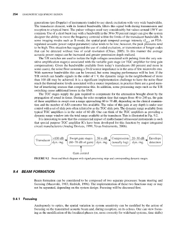
The TGC stages supply the gain required to compensate for the attenuation brought about by the
propagation of sound in tissue. During the echo reception time that ranges from 40 to 240 μs, the gain
of these amplifiers is swept over a range approaching 60 to 70 dB, depending on the clinical examina-
tion and the number of A/D converter bits available. The value of this gain at any depth is under user
control with a set of slide pots often referred to as the TGC slide pots. The dynamic range available from
typical TGC amplifiers is in the order of 60 dB. One can think of the TGC amplifiers as providing a
dynamic range window into the total range available at the transducer. This is illustrated in Fig. 9.2.
It is interesting to note that the commercial impact of multichannel ultrasound instruments is such
that special purpose TGC amplifier ICs have been developed for this function by major integrated
circuit manufacturers (Analog Devices, 1999; Texas Instruments, 2006).

>100 dB Swept gain stages 50 + dB Compression 20–30 dB Envelope
Transducer
dyn. rng. (60–70 dB of gain) dyn. rng. (usually log) dyn. rng. detection

Gain control
FIGURE 9.2 Front-end block diagram with signal-processing steps and corresponding dynamic ranges.

9.4 BEAM FORMATION

Beam formation can be considered to be composed of two separate processes: beam steering and
focusing (Macovski, 1983; Hedrick, 1996). The implementation of these two functions may or may
not be separated, depending on the system design. Focusing will be discussed first.

9.4.1 Focusing

Analogously to optics, the spatial variation in system sensitivity can be modified by the action of
focusing on the transmitted acoustic beam and, during reception, on its echoes. One can view focus-
ing as the modification of the localized phases (or, more correctly for wideband systems, time shifts)