Page 280 - Biomedical Engineering and Design Handbook Volume 2, Applications

258 DIAGNOSTIC EQUIPMENT DESIGN

60
30-mm focus
40 50-mm focus
Depth along transducer, mm –20 80-mm focus
20

0

–40 50-mm focus
30-mm focus
–60
0 50 100 150 200
Depth, mm
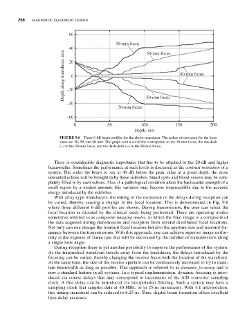
FIGURE 9.6 Three 6-dB beam profiles for the above transducer. The radius of curvature for the three
cases are 30, 50, and 80 mm. The graph with a solid line corresponds to the 30-mm focus, the dot-dash
(.-) to the 50-mm focus, and the dash-dash (--) to the 80-mm focus.

There is considerable diagnostic importance that has to be attached to the 20-dB and higher
beamwidths. Sometimes the performance at such levels is discussed as the contrast resolution of a
system. The wider the beam is, say at 40 dB below the peak value at a given depth, the more
unwanted echoes will be brought in by these sidelobes. Small cysts and blood vessels may be com-
pletely filled in by such echoes. Also, if a pathological condition alters the backscatter strength of a
small region by a modest amount, this variation may become imperceptible due to the acoustic
energy introduced by the sidelobes.
With array-type transducers, the timing of the excitation or the delays during reception can
be varied, thereby causing a change in the focal location. This is demonstrated in Fig. 9.6
where three different 6-dB profiles are shown. During transmission, the user can select the
focal location as dictated by the clinical study being performed. There are operating modes
sometimes referred to as composite imaging modes, in which the final image is a composite of
the data acquired during transmission and reception from several distributed focal locations.
Not only can one change the transmit focal location but also the aperture size and transmit fre-
quency between the transmissions. With this approach, one can achieve superior image unifor-
mity at the expense of frame rate that will be decreased by the number of transmissions along
a single look angle.
During reception there is yet another possibility to improve the performance of the system.
As the transmitted wavefront travels away from the transducer, the delays introduced by the
focusing can be varied, thereby changing the receive focus with the location of the wavefront.
At the same time, the size of the receive aperture can be continuously increased to try to main-
tain beamwidth as long as possible. This approach is referred to as dynamic focusing and is
now a standard feature in all systems. In a typical implementation, dynamic focusing is intro-
duced via course delays that may correspond to increments of the A/D converter sampling
clock. A fine delay can be introduced via interpolation filtering. Such a system may have a
sampling clock that samples data at 40 MHz, or in 25-ns increments. With 4:1 interpolation,
this timing increment can be reduced to 6.25 ns. Thus, digital beam formation offers excellent
time delay accuracy.