Page 297 - Biomedical Engineering and Design Handbook Volume 2, Applications

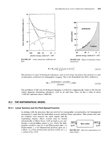
THE PRINCIPLES OF X-RAY COMPUTED TOMOGRAPHY 275

3
3
photon energy (units keV × 10 ) photon energy (units keV × 10 )
FIGURE 10.7 Linear attenuation coefficients for FIGURE 10.8 Region of dominant attenua-
H O. tion process.
2
Φ = Φ exp ( ∫ ∫ μ ( , ) dl d λ )
λ
−
r
0 λ l (10.23)
The presence of water in biological substances, such as soft tissue, has lead to the creation of a unit
of attenuation coefficient for tomographic imaging. This is the Hounsfield unit (HU), defined as
μ( substance − μ) ( water)
HU = ×1000 (10.24)
μ( water)
The usefulness of this unit for biological imaging is evident by comparing the values in HU for the
widely disparate attenuating substances, such as air and bone. Here, air has a value of about
−1000 HU and bone about +1000 HU.

10.3 THE MATHEMATICAL MODEL

10.3.1 Linear Systems and the Point-Spread Function

In dealing with the processes that are involved in tomographic reconstruction, the fundamental
assumption is made that the individual systems perform linear operations. This ensures that sim-
ple relations exist between the input signals and the
responding outputs. These systems may be treated
schematically as black boxes, with an input g (u), pro-
in
ducing a corresponding output g (u), where the inde-
out
pendent variable u may be a one-dimensional time t, or
displacement x, a two-dimensional position upon an x,
y plane, or a three-dimensional position within an x, y, FIGURE 10.9 Black box representation of a
z volume (Fig. 10.9). linear system.