Page 300 - Biomedical Engineering and Design Handbook Volume 2, Applications

278 DIAGNOSTIC EQUIPMENT DESIGN

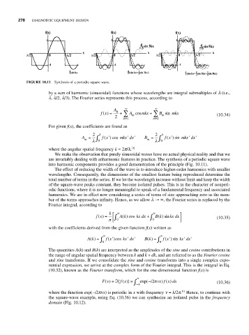
FIGURE 10.11 Synthesis of a periodic square wave.

by a sum of harmonic (sinusoidal) functions whose wavelengths are integral submultiples of l (i.e.,
l, l/2, l/3). The Fourier series represents this process, according to

A ∞ ∞
fx() = 0 + ∑ A cos mkx + ∑ B sin mkx
2 m m (10.34)
m=1 m=1
For given f(x), the coefficients are found as
2 λ 2 λ λ
′
′
A = ∫ f x′ cos mkx dx′ B = ∫ f x′ sin mkx dx′
()
()
m
λ 0 m λ 0
where the angular spatial frequency k = 2p/l. 10
We make the observation that purely sinusoidal waves have no actual physical reality and that we
are invariably dealing with anharmonic features in practice. The synthesis of a periodic square wave
into harmonic components provides a good demonstration of the principle (Fig. 10.11).
The effect of reducing the width of the wave is to introduce higher-order harmonics with smaller
wavelengths. Consequently, the dimensions of the smallest feature being reproduced determine the
total number of terms in the series. If we let the wavelength increase without limit and keep the width
of the square-wave peaks constant, they become isolated pulses. This is in the character of nonperi-
odic functions, where it is no longer meaningful to speak of a fundamental frequency and associated
harmonics. We are in effect now considering a series of terms of size approaching zero as the num-
ber of the terms approaches infinity. Hence, as we allow l →∞, the Fourier series is replaced by the
Fourier integral, according to
1 ⎡ ∞ ∞ ⎤
f x() = ⎢∫ A k) cos kx dx + ∫ B k) sin kx dx (10.35)
(
(
π ⎣ 0 0 ⎥ ⎦
with the coefficients derived from the given function f(x) written as
∞ ∞
′
( ′
′
A k() = ∫ 0 0 fx )cos kx dx′ B k() = ∫ 0 fx ) sin kx dx′
( ′
The quantities A(k) and B(k) are interpreted as the amplitudes of the sine and cosine contributions in
the range of angular spatial frequency between k and k + dk, and are referred to as the Fourier cosine
and sine transforms. If we consolidate the sine and cosine transforms into a single complex expo-
nential expression, we arrive at the complex form of the Fourier integral. This is the integral in Eq.
(10.32), known as the Fourier transform, which for the one-dimensional function f(x) is
∞
Fv) =ℑ { f x)} = ∫ −∞ exp(− i2π vx f x dx (10.36)
(
)
(
(
)
11
where the function exp(−i2pnx) is periodic in x with frequency n = k/2p. Hence, to continue with
the square-wave example, using Eq. (10.36) we can synthesize an isolated pulse in the frequency
domain (Fig. 10.12).