Page 299 - Biomedical Engineering and Design Handbook Volume 2, Applications

THE PRINCIPLES OF X-RAY COMPUTED TOMOGRAPHY 277

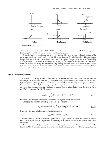
FIGURE 10.10 The convolution process.

This has the shorthand notation f**h = h**f, where ** denotes convolution with double integration.
Similarly, f*h = h*f denotes convolution with single integration.
A physical description of convolution can be expressed in terms of graphical manipulation of the
one-dimensional function f(x′) (Fig. 10.10). Here, the function h(x′) is folded by taking the mirror
image about the ordinate axis, a displacement h(−x′) is applied along the abscissa axis, followed by
a multiplication of the shifted function h(x − x′) by f(x′). The convolution at location x is then deter-
mined by integration along the abscissa axis, by finding the area under the product of h(x − x′) and
f(x′). The result of convolution will be the same if the role of the two functions is reversed, that is
whether h(x′) or f(x′) is folded and shifted.

10.3.2 Frequency Domain
The method of resolving the input into a linear combination of d functions presents a framework for
the analysis of linear shift-invariant systems in cartesian space. However, solutions involve the mul-
tiple integration of the product of functions and are cumbersome to carry out in practice. Since d
functions are not the only form of input signal decomposition, it is expedient to examine the super-
position of complex exponential functions as a possible alternative. In this case the input g (u) =
in
exp(i2pk ⋅u), so that Eq. (10.29) becomes
∞
k u′
g out () = ∫ −∞ p(u′ − ) u exp(+ i2π ⋅⋅ ) du′ (10.31)
u
where u is the independent variable vector and k is a given real number vector.
Changing the variables according to u′′ = u − u′, we have
∞
d ′′
k u′′
k
u
g ( ) = exp( i2π ⋅⋅ ) u ∫ p(u′′ ) exp(− i2π ⋅⋅ ) u
u
out −∞ (10.32)
Since the integrand is independent of u, this reduces to
u
u
g out () = constant × g () (10.33)
in
This indicates that passing a complex exponential through a linear shift-invariant system is equiva-
lent to multiplying it by a complex factor depending on k, which in effect is the transfer function of
the system.
The result [Eq. (10.32)] allows us to consider each image to be constructed from a series of sinusoidal
functions. This leads to the concept that a function f(x), having a spatial period l, can be synthesized