Page 301 - Biomedical Engineering and Design Handbook Volume 2, Applications

THE PRINCIPLES OF X-RAY COMPUTED TOMOGRAPHY 279

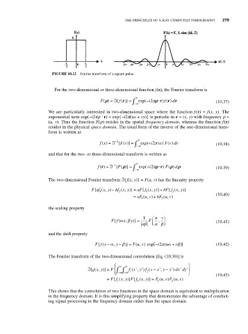
FIGURE 10.12 Fourier transform of a square pulse.

For the two-dimensional or three-dimensional function f(r), the Fourier transform is
∞
ρ
F( ) =ℑ f { ( )} = ∫ −∞ exp(− i2π ρρ r f ) ( ) dr (10.37)
⋅⋅
ρ
r
r
We are particularly interested in two-dimensional space where the function f(r) = f(x, y). The
exponential term exp(−i2pr ⋅ r) = exp{-i2p(ux + vy)} is periodic in r = (x, y) with frequency ρ =
(u, v). Thus the function F(r) resides in the spatial frequency domain, whereas the function f(r)
resides in the physical space domain. The usual form of the inverse of the one-dimensional trans-
form is written as
∞
fx) =ℑ −1 { F v)} = ∫ exp(+ i2π vx F v dv (10.38)
(
(
(
)
)
−∞
and that for the two- or three-dimensional transform is written as
∞
ρ
ρ
f ( ) =ℑ −1 { F( )} = ∫ −∞ exp(+ i2 ρρ⋅⋅ ) r F( ) dρρ (10.39)
π
ρ
ρ
r
The two-dimensional Fourier transform ℑ{f(x, y)} = F(u, v) has the linearity property
F af x y,) + bfx y,)} = aF f x y,)}+ bF fx y,)}
{
(
{
(
}
{
(
(
2
1
1
2
(10.40)
u
v
u
= aF 1 (, ) + bF 2 (, )
v
the scaling property
1 ⎛ uv ⎞
Ff{(α x, β y)} = F ⎜ , ⎟ (10.41)
αβ ⎝ α β⎠
and the shift property
Ff x −α y , − β )} = F u v) exp[− π α + v )] (10.42)
β
2
u (
(
(
,
i
{
The Fourier transform of the two-dimensional convolution [Eq. (10.30)] is
′
− ′
(,
,
ℑ{gx y) } = F ∫ −∞ { ∞ ∫ ∞ f ( ′ x y f x, ′) ( − ′ x y y dxxdy′ }
)
1
2
−∞
(10.43)
= Ff x y Ff x y ={( , )} { ( , )} F u v F u v , )
( , )
(
1 2 1 2
This shows that the convolution of two functions in the space domain is equivalent to multiplication
in the frequency domain. It is this simplifying property that demonstrates the advantage of conduct-
ing signal processing in the frequency domain rather than the space domain.