Page 306 - Biomedical Engineering and Design Handbook Volume 2, Applications

284 DIAGNOSTIC EQUIPMENT DESIGN

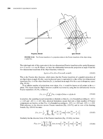
FIGURE 10.16 The Fourier transform of a projection relates to the Fourier transform of the object along
a radial line.

The right-hand side of this expression is the two-dimensional Fourier transform at the spatial frequency
(u = w cos q, v = w sin q). Hence, we have the relationship between the projection at angle q and the
two-dimensional transform of the object function, written as
S w() = Fw θ) = Fwcos θ, wsin θ) (10.63)
(
(,
θ
This is the Fourier slice theorem, which states that the Fourier transform of a parallel projection of
an object taken at angle q to the x axis in physical space is equivalent to a slice of the two-dimensional
transform F(u, v) of the object function f(x, y), inclined at an angle q to the u axis in frequency space
(Fig. 10.16).
If an infinite number of projections were taken, F(u, v) would be known at all points in the u, v
plane. This means that the object function could be recovered by using the two-dimensional inverse
Fourier transform (10.39), written as
∞ ∞
fx y) = ∫ −∞ ∫ −∞ F u v) exp[+ i2π ( ux vy du dv (10.64)
+
,
(
(
,
]
)
In practice, the sampling in each projection is limited, so that f(x, y) is bounded according to −A/2 <
x < A/2 and −A/2 < y < A/2. Also, physical limitations ensure that only a finite number of Fourier
components are known, so that F(u, v) is bounded according to −N/2 < u < N/2 and −N/2 < v < N/2.
With reference to the discrete inverse Fourier transform [Eq. (10.47)], and in view of the limiting
bounds, Eq. (10.64) becomes
1 N/2 N/2 ⎛ m n ⎞ ⎡ ⎛ m n ⎞ ⎤
fx y) = 2 ∑ ∑ F , exp ⎢ i + 2π x + y ⎥ (10.65)
(,
A ⎝ A A ⎠ ⎣ ⎝ A A ⎠ ⎥ ⎦
2
m =−N n =−N/2
/
Similarly for the discrete form of the Fourier transform [Eq. (10.46)], we have
⎫
1 M −1 ⎧ ⎪ 1 N−1 ⎡ 2π ⎤⎪ ⎡ 2π ⎤
Fu v) = ∑ ⎨ ∑ fm n) exp − i nv ⎬ exp −i mu (10.66)
(,
(
,
M ⎩ ⎩ ⎪ N ⎢ ⎣ N ⎥ ⎦ ⎪ ⎢ ⎣ M ⎥ ⎦
m =0 n=0 ⎭