Page 308 - Biomedical Engineering and Design Handbook Volume 2, Applications

286 DIAGNOSTIC EQUIPMENT DESIGN

and the estimate is a vertical wedge (Fig. 10.18b) with the same mass as the pie wedge. The approx-
imation can be made increasingly accurate the greater the number of projections taken.
A formal description of the filtered back-projection process is best served by expressing the object
function f(x, y) defined in Eq. (10.64), in an alternative coordinate system. Here, the rectangular coordi-
nate system in the frequency domain (u, v) is exchanged for the polar coordinate system (w, q), so that

2π ∞
θ
f x y) = ∫ 0 ∫ ∫ 0 F w, ) exp[+ π w x cos + ysin )] w dw dθ (10.67)
θ
θ
(
,
(
2
(
i
given that u = cosq and v = w sinq. Splitting the integral into two parts, in the ranges 0 to p and p to
2p, using the property F(w, q + p) = F(−w, q), and substituting from Eqs. (10.59) and (10.62), we get
π ⎡ ∞ ⎤
fx y) = ∫ 0 ⎢∫ S ( w w| exp(+ π wr dw dθ (10.68)
i
2
|
)
)
(
,
⎥
θ
⎦
⎣ −∞
If we write the integral inside the straight brackets [] as
∞
Qr) = ∫ S w w| exp(+ i π wr dw (10.69)
(
)
)
2
|
(
θ −∞ θ
the object function, for projections over 180°, becomes
π
θ
fx y) = ∫ Q x cos + ysin ) dθ (10.70)
θ
(,
(
θ
0
The function Q (r) is a filtered projection so that Eq. (10.70) represents a summation of back-
q
projections from the filtered projections. This means that a particular Q (r) will contribute the same
q
value at every point (x, y) in the reconstructed image plane that lies on the line defined by (r, q)
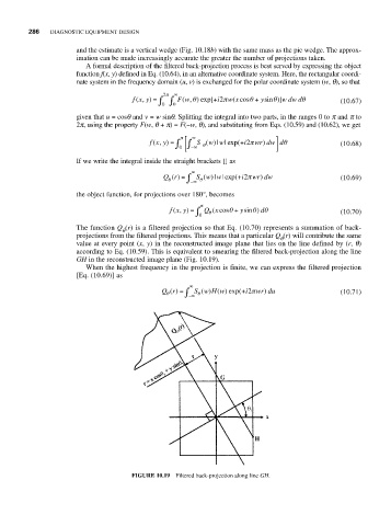
according to Eq. (10.59). This is equivalent to smearing the filtered back-projection along the line
GH in the reconstructed image plane (Fig. 10.19).
When the highest frequency in the projection is finite, we can express the filtered projection
[Eq. (10.69)] as
∞
Qr) = ∫ −∞ S w H w() exp(+ i π wr du (10.71)
)
2
()
(
θ
θ
FIGURE 10.19 Filtered back-projection along line GH.