Page 307 - Biomedical Engineering and Design Handbook Volume 2, Applications

THE PRINCIPLES OF X-RAY COMPUTED TOMOGRAPHY 285

for u = 0, . . . , M − 1; v = 0, . . . , N − 1. The expression within the curly brackets {} is the one-
dimensional finite Fourier transform of the mth row of the projected image and can be computed using
the fast Fourier transform (FFT) algorithm. To compute F(u, v), each row in the image is replaced by
its one-dimensional FFT, followed by the one-dimensional FFT of each column. The spatial resolu-
tion of the reconstructed f(x, y), in the plane of the projection, is determined by the range N of Fourier
components used.
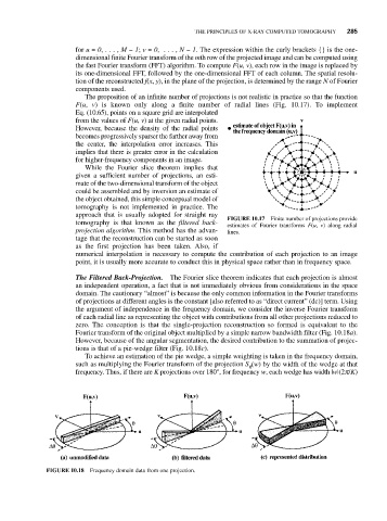
The proposition of an infinite number of projections is not realistic in practice so that the function
F(u, v) is known only along a finite number of radial lines (Fig. 10.17). To implement
Eq. (10.65), points on a square grid are interpolated
from the values of F(u, v) at the given radial points.
However, because the density of the radial points
becomes progressively sparser the farther away from
the center, the interpolation error increases. This
implies that there is greater error in the calculation
for higher-frequency components in an image.
While the Fourier slice theorem implies that
given a sufficient number of projections, an esti-
mate of the two-dimensional transform of the object
could be assembled and by inversion an estimate of
the object obtained, this simple conceptual model of
tomography is not implemented in practice. The
approach that is usually adopted for straight ray FIGURE 10.17 Finite number of projections provide
tomography is that known as the filtered back- estimates of Fourier transforms F(u, v) along radial
projection algorithm. This method has the advan- lines.
tage that the reconstruction can be started as soon
as the first projection has been taken. Also, if
numerical interpolation is necessary to compute the contribution of each projection to an image
point, it is usually more accurate to conduct this in physical space rather than in frequency space.

The Filtered Back-Projection. The Fourier slice theorem indicates that each projection is almost
an independent operation, a fact that is not immediately obvious from considerations in the space
domain. The cautionary “almost” is because the only common information in the Fourier transforms
of projections at different angles is the constant [also referred to as “direct current” (dc)] term. Using
the argument of independence in the frequency domain, we consider the inverse Fourier transform
of each radial line as representing the object with contributions from all other projections reduced to
zero. The conception is that the single-projection reconstruction so formed is equivalent to the
Fourier transform of the original object multiplied by a simple narrow bandwidth filter (Fig. 10.18a).
However, because of the angular segmentation, the desired contribution to the summation of projec-
tions is that of a pie-wedge filter (Fig. 10.18c).
To achieve an estimation of the pie wedge, a simple weighting is taken in the frequency domain,
such as multiplying the Fourier transform of the projection S (w) by the width of the wedge at that
q
frequency. Thus, if there are K projections over 180°, for frequency w, each wedge has width |w|(2p/K)

FIGURE 10.18 Frequency domain data from one projection.