Page 312 - Biomedical Engineering and Design Handbook Volume 2, Applications

290 DIAGNOSTIC EQUIPMENT DESIGN

Hence, the reconstructed object function according to Eq. (10.77) may be written as
1 2π D 2 ∞ ⎛ Dr ⎞ D
frs) = ∫ SO 2 ∫ Rp h SO − p SO dp dβ
(,
()
β
2 0 ( D − s) −∞ ⎜ ⎝ D − s ⎟ ⎟ ⎠ 2 2 (10.82)
SO SO D SO + p
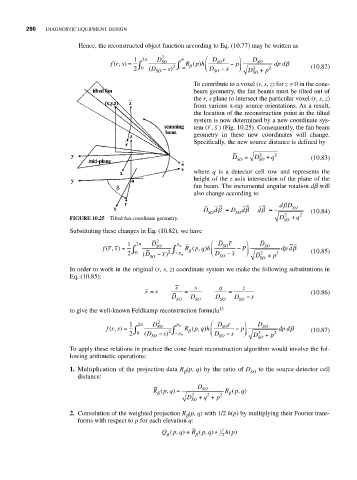
To contribute to a voxel (r, s, z) for z = / 0 in the cone-
beam geometry, the fan beams must be tilted out of
the r, s plane to intersect the particular voxel (r, s, z)
from various x-ray source orientations. As a result,
the location of the reconstruction point in the tilted
system is now determined by a new coordinate sys-
– –
tem (r , s ) (Fig. 10.25). Consequently, the fan beam
geometry in these new coordinates will change.
Specifically, the new source distance is defined by
D = D 2 + q 2 (10.83)
SO SO
where q is a detector cell row and represents the
height of the z axis intersection of the plane of the
fan beam. The incremental angular rotation db will
also change according to
β
dD
D dβ = D dβ dβ = SO (10.84)
SO SO 2 2
FIGURE 10.25 Tilted fan coordinate geometry. D SO + q
Substituting these changes in Eq. (10.82), we have
1 2π D 2 SO p m ⎛ Dr ⎞ ⎞ D SO
SO
fr s) = ∫ 2 ∫ Rp q h ) ⎜ − P ⎟ dp dβ
(,
(,
β
2 0 ( D − s) − p m ⎝ D − s ⎠ 2 2 (10.85)
SO SO D SO + p
In order to work in the original (r, s, z) coordinate system we make the following substitutions in
Eq. (10.85):
s s q z
r = r = = (10.86)
D D D D − s
SO SO SO SO
to give the well-known Feldkamp reconstruction formula 13
1 2π D 2 p m ⎛ Dr ⎞ D
frs) = ∫ SO 2 ∫ Rp q h ) ⎜ SO − p p ⎟ SO dp dβ (10.87)
(,
(,
β
2 0 ( D SO − s) − p m ⎝ D SO − s ⎠ D SO + p 2
2
To apply these relations in practice the cone-beam reconstruction algorithm would involve the fol-
lowing arithmetic operations:
1. Multiplication of the projection data R (p, q) by the ratio of D to the source-detector cell
b SO
distance:
D
Rp q) = SO Rp q)
(,
(,
β
β
2
2
D SO + q + p 2
2. Convolution of the weighted projection R (p, q) with 1/2 h(p) by multiplying their Fourier trans-
b
forms with respect to p for each elevation q:
Qp q) = (, 1 h p()
(,
β R p q) * 2
β