Page 316 - Biomedical Engineering and Design Handbook Volume 2, Applications

294 DIAGNOSTIC EQUIPMENT DESIGN

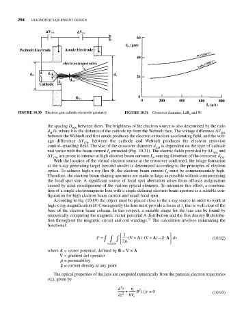
FIGURE 10.30 Electron gun cathode-electrode geometry. FIGURE 10.31 Crossover diameter, LaB and W.
6
the spacing D between them. The brightness of the electron source is also determined by the ratio
WA
d /h, where h is the distance of the cathode tip from the Wehnelt face. The voltage difference ΔV
W WA
between the Wehnelt and first anode produces the electron extraction-accelerating field, and the volt-
age difference ΔV between the cathode and Wehnelt produces the electron emission
CW
control–retarding field. The size of the crossover diameter d is dependent on the type of cathode
CO
and varies with the beam current I extracted (Fig. 10.31). The electric fields provided by ΔV and
0 WA
ΔV are prone to interact at high electron beam currents I , causing distortion of the crossover d .
CW 0 CO
With the location of the virtual electron source at the crossover confirmed, the image formation
at the x-ray generating target (second anode) is determined according to the principles of electron
optics. To achieve high x-ray flux Φ, the electron beam current I must be commensurately high.
0
Therefore, the electron beam shaping apertures are made as large as possible without compromising
the focal spot size. A significant source of focal spot aberration arises from off-axis astigmatism
caused by axial misalignment of the various optical elements. To minimize this effect, a combina-
tion of a single electromagnetic lens with a single defining electron beam aperture is a suitable con-
figuration for high electron beam current and small focal spot.
According to Eq. (10.89) the object must be placed close to the x-ray source in order to work at
high x-ray magnification M. Consequently the lens must provide a focus at z that is well clear of the
i
base of the electron beam column. In this respect, a suitable shape for the lens can be found by
numerically computing the magnetic vector potential A distribution and the flux density B distribu-
tion throughout the magnetic circuit and coil windings. 21 The calculation involves minimizing the
functional:
⎧ 1 ⎫
F = ∫ ∫ ⎨ ∫ ( ∇ × ) ⋅ ∇ × ) J A dv (10.92)
− ⋅ ⎬
A
A
(
volume ⎩ 2μ ⎭
where A = vector potential, defined by B =∇× A
∇= gradient del operator
m = permeability
J = current density at any point
The optical properties of the lens are computed numerically from the paraxial electron trajectories
r(z), given by
2
dr + η Bz r =() 0
2
dz 2 8 V r (10.93)