Page 309 - Biomedical Engineering and Design Handbook Volume 2, Applications

THE PRINCIPLES OF X-RAY COMPUTED TOMOGRAPHY 287

where
⎧1 | < w | < W
=
Hw() | w b w() and b w() = ⎨
|
w w
⎩ 0 otherwise
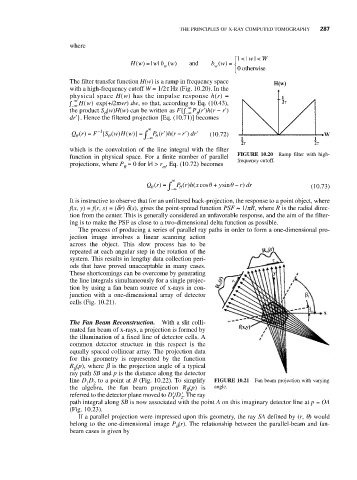
The filter transfer function H(w) is a ramp in frequency space
with a high-frequency cutoff W = 1/2t Hz (Fig. 10.20). In the
physical space H(w) has the impulse response h(r) =
∞
∫ −∞ H(w) exp(+i2pwr) dw, so that, according to Eq. (10.43),
∞
q q
the product S (w)H(w) can be written as F{∫ −∞ P (r′)h(r − r′)
dr′}. Hence the filtered projection [Eq. (10.71)] becomes
∞
−1
Qr() = F { S w H w)} = ∫ −∞ P r h r r dr′ (10.72)
) ′
−
( ′
(
)
(
)
(
θ
θ
θ
which is the convolution of the line integral with the filter
FIGURE 10.20 Ramp filter with high-
function in physical space. For a finite number of parallel frequency cutoff.
projections, where P = 0 for |r| > r , Eq. (10.72) becomes
q m
∞
θ
Qr() = ∫ −∞ P r h x cos + ysin − r dr (10.73)
θ
()
)
(
θ
θ
It is instructive to observe that for an unfiltered back-projection, the response to a point object, where
f(x, y) = f(r, s) = (dr) d(s), gives the point-spread function PSF ≈ 1/pR, where R is the radial direc-
tion from the center. This is generally considered an unfavorable response, and the aim of the filter-
ing is to make the PSF as close to a two-dimensional delta function as possible.
The process of producing a series of parallel ray paths in order to form a one-dimensional pro-
jection image involves a linear scanning action
across the object. This slow process has to be
repeated at each angular step in the rotation of the
system. This results in lengthy data collection peri-
ods that have proved unacceptable in many cases.
These shortcomings can be overcome by generating
the line integrals simultaneously for a single projec-
tion by using a fan beam source of x-rays in con-
junction with a one-dimensional array of detector
cells (Fig. 10.21).
The Fan Beam Reconstruction. With a slit colli-
mated fan beam of x-rays, a projection is formed by
the illumination of a fixed line of detector cells. A
common detector structure in this respect is the
equally spaced collinear array. The projection data
for this geometry is represented by the function
R (p), where b is the projection angle of a typical
b
ray path SB and p is the distance along the detector
line D D to a point at B (Fig. 10.22). To simplify FIGURE 10.21 Fan beam projection with varying
1 2
the algebra, the fan beam projection R b (p) is angle.
referred to the detector plane moved to D′/D′. The ray
1 2
path integral along SB is now associated with the point A on this imaginary detector line at p = OA
(Fig. 10.23).
If a parallel projection were impressed upon this geometry, the ray SA defined by (r, q) would
belong to the one-dimensional image P (r). The relationship between the parallel-beam and fan-
q
beam cases is given by