Page 305 - Biomedical Engineering and Design Handbook Volume 2, Applications

THE PRINCIPLES OF X-RAY COMPUTED TOMOGRAPHY 283

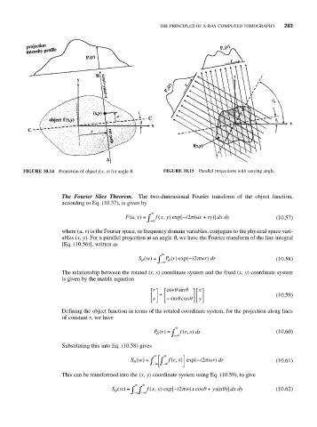
FIGURE 10.14 Projection of object f(x, y) for angle q. FIGURE 10.15 Parallel projections with varying angle.

The Fourier Slice Theorem. The two-dimensional Fourier transform of the object function,
according to Eq. (10.37), is given by
∞
Fu v) = ∫ −∞ f x y) exp[− i2π ( ux vy dx dy (10.57)
+
(
,
,
(
)
]
where (u, v) is the Fourier space, or frequency domain variables, conjugate to the physical space vari-
ables (x, y). For a parallel projection at an angle q, we have the Fourier transform of the line integral
[Eq. (10.56)], written as
∞
Sw) = ∫ P r) exp(− i π wr dr (10.58)
(
)
2
(
θ θ
−∞
The relationship between the rotated (r, s) coordinate system and the fixed (x, y) coordinate system
is given by the matrix equation
θ
r ⎡ ⎤ ⎡ cos sinθ ⎤ x ⎡ ⎤
⎢ ⎥ = ⎢ ⎥⎢ ⎥ (10.59)
θ
s ⎣ ⎦ ⎣ −sin cosθ ⎦ y ⎣ ⎦
Defining the object function in terms of the rotated coordinate system, for the projection along lines
of constant r, we have
∞
Pr() = ∫ −∞ f r s ds (10.60)
)
(,
θ
Substituting this into Eq. (10.58) gives
∞ ⎡ ∞ ⎤
∫
Sw) = ∫ −∞ ⎣ ⎢ −∞ f r s) exp(− i π wr dr (10.61)
)
2
,
(
(
θ
⎦ ⎥
This can be transformed into the (x, y) coordinate system using Eq. (10.59), to give
∞ ∞
θ
Sw) = ∫ − −∞ ∫ −∞ f x y) exp[− i π w x cos + ysin θ)] dx dy (10.62)
(
,
2
(
(
θ