Page 310 - Biomedical Engineering and Design Handbook Volume 2, Applications

288 DIAGNOSTIC EQUIPMENT DESIGN

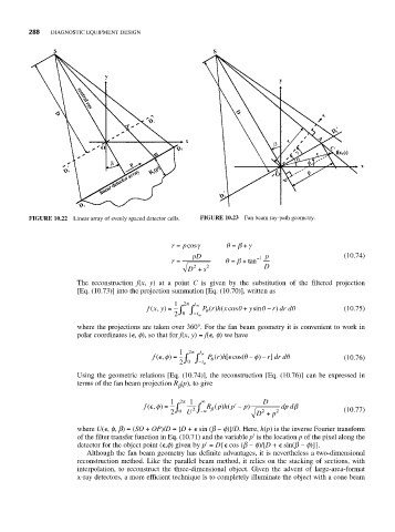
FIGURE 10.22 Linear array of evenly spaced detector cells. FIGURE 10.23 Fan beam ray-path geometry.

+
r = cosγ θ = β γ
p
pD −1 p (10.74)
r = θ = β + tan
2
D + s 2 D
The reconstruction f(x, y) at a point C is given by the substitution of the filtered projection
[Eq. (10.73)] into the projection summation [Eq. (10.70)], written as
1 2π t m
θ
fx y) = ∫ ∫ ∫ P r h x cos + ysin − r dr dθ (10.75)
θ
(,
(
)
(
)
θ
2 0 − t m
where the projections are taken over 360°. For the fan beam geometry it is convenient to work in
polar coordinates ( , f), so that for f(x, y) = f( , f) we have
1 2 π t m

f (, ) = ∫ ∫ P r h[ cos(θ φ − r dr dθ (10.76)
−
φ

)
)
(
]
θ
2 0 − t m
Using the geometric relations [Eq. (10.74)], the reconstruction [Eq. (10.76)] can be expressed in
terms of the fan beam projection R (p), to give
b
1 2 π 1 ∞ D
f (, ) φ = ∫ 2 ∫ Rp h p ( ′ − p) dp dβ

( )
β
2
2 0 U −∞ D + p 2 (10.77)
where U( , f, b) = (SO + OP)/D = [D + sin (b − f)]/D. Here, h(p) is the inverse Fourier transform
of the filter transfer function in Eq. (10.71) and the variable p′ is the location p of the pixel along the
detector for the object point ( ,f) given by p′= D{ cos (b − f)/[D + sin(b − f)]}.
Although the fan beam geometry has definite advantages, it is nevertheless a two-dimensional
reconstruction method. Like the parallel beam method, it relies on the stacking of sections, with
interpolation, to reconstruct the three-dimensional object. Given the advent of large-area-format
x-ray detectors, a more efficient technique is to completely illuminate the object with a cone beam