Page 443 - Cam Design Handbook

THB13 9/19/03 7:56 PM Page 431

CAM SYSTEM DYNAMICS—RESPONSE 431

envelope will be found at some limiting value of m. In this case the resulting design should
be nearly optimal.

13.6.5 Constant Velocity Convolution
As an illustration of fixed-convolution let us consider w(1,b,q) to be the velocity curve for
constant velocity. Then
q
v ( d,,bq ) = (2 b ) v d ( ,b 2,t ) d ◊ t 0 , £ £ b 2
q
i+1
i Ú 0
b 2
= (2 b ) vd ( ,b 2,t ) d ◊ t ,b 2 £ £ .q b (13.72)
- Ú qb 2 i
The postconvolution acceleration curve is obtained by differentiation of Eq. (13.72)
a ( d,,bq ) = (2 b ) v d ( ,b 2,q ) 0, ££ b 2
q
i+1 i
= (2 b ) vd ( ,b 2,q - b ) 2 ,b 2 ££ .q b (13.73)
i
In dimensionless form
*
v () = 2 Ú 0 2h v () t d 0 ££1 2
t
h
*
,
h
i+1
i
1
*
d 1 2
= 2 v () tt , ££1h (13.74)
- Ú 2h 1 i
a () = 4 * ) 0, ££1 2
h
* h
v (2h
i+1
i
=-4 * - ) 1 0 , ££1.h (13.75)
v (2h
i
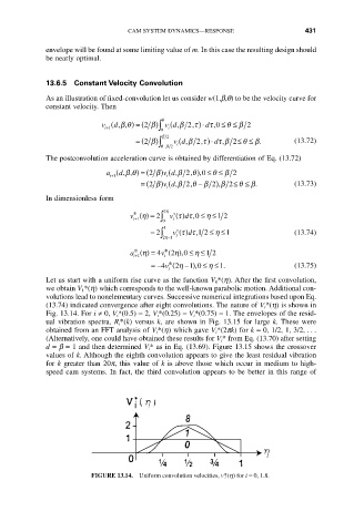
Let us start with a uniform rise curve as the function V 0 *(h). After the first convolution,
we obtain V 1*(h) which corresponds to the well-known parabolic motion. Additional con-
volutions lead to nonelementary curves. Successive numerical integrations based upon Eq.
(13.74) indicated convergence after eight convolutions. The nature of V i *(h) is shown in
Fig. 13.14. For i π 0, V i*(0.5) = 2, V i*(0.25) = V i*(0.75) = 1. The envelopes of the resid-
ual vibration spectra, R i*(k) versus k, are shown in Fig. 13.15 for large k. These were
obtained from an FFT analysis of V i *(h) which gave V i *(2pk) for k = 0, 1/2, 1, 3/2,...
(Alternatively, one could have obtained these results for V i* from Eq. (13.70) after setting
d = b = 1 and then determined V i* as in Eq. (13.69). Figure 13.15 shows the crossover
values of k. Although the eighth convolution appears to give the least residual vibration
for k greater than 20p, this value of k is above those which occur in medium to high-
speed cam systems. In fact, the third convolution appears to be better in this range of

FIGURE 13.14. Uniform convolution velocities, v* i (h) for i = 0, 1.8.