Page 171 - Carbonate Sedimentology and Sequence Stratigraphy

162 WOLFGANG SCHLAGER

matician Georg Cantor in the nineteenth century. The fractal Koch curve, the coastline is a very wiggly curve with a fine
is constructed by erasing the middle third of a line segment structure in a wide range of scales. We will see below that
and again, as with the Koch curve, repeating the initial op- its fractal dimension is between 1 and 2, again similar to the
eration an infinite number of times. The result is a fractal set Koch curve. Two important differences between this natural
with a dimension between zero and one, the Euclidean di- object and the Koch curve should be noted: First, the coast-
mensions of a point and a line respectively. The topological line is a fractal only in a statistical sense. Magnifying part
dimension of the Cantor set would be zero. of the coast to the scale of the entire feature will produce
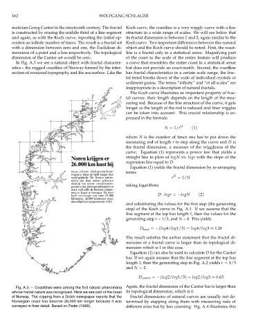
In Fig. A.3 we see a natural object with fractal character- a curve that resembles the entire coast in a statistical sense
istics – the rugged coastline of Norway formed by the inter- but does not provide an exact match. Second, the coastline
section of erosional topography and the sea surface. Like the has fractal characteristics in a certain scale range, the frac-
tal trend breaks down at the scale of individual crystals or
sediment grains. The terms “infinity” and “at all scales” are
inappropriate in a description of natural fractals.
The Koch curve illustrates an important property of frac-
tal curves: their length depends on the length of the mea-
suring rod. Because of the fine structure of the curve, it gets
longer as the length of the rod is reduced and finer wiggles
can be taken into account. This crucial relationship is ex-
pressed in the formula

N = 1/r D (1)
where N is the number of times one has to put down the
measuring rod of length r to step along the curve and D is
the fractal dimension, a measure of the wiggliness of the
curve. Equation (1) represents a power law that yields a
straight line in plots of logN vs. logr with the slope of the
regression line equal to D.
Equation (1) yields the fractal dimension by re-arranging
terms
D
r = 1/N
taking logarithms

D · logr = −logN (2)
and substituting the values for the first step (the generating
step) of the Koch curve in Fig. A.1. If we assume that the
line segment at the top has length 1, then the values for the
generating step r =1/3, and N = 4. This yields

D koch = −(log4/log1/3)= log4/log3 ≈ 1.26
The result satisfies the earlier statement that the fractal di-
mension of a fractal curve is larger than its topological di-
mension which is 1 in this case.
Equation (1) can also be used to calculate D for the Cantor
bar. If we again assume that the line segment at the top has
length 1, then the generating step in Fig. A.2 yields r = 1/3
and N = 2.

D cantor = −(log2/log1/3)= log2/log3 ≈ 0.63

Fig. A.3.— Coastlines were among the first natural phenomena Again, the fractal dimension of the Cantor bar is larger than
whose fractal nature was recognized. Here we see part of the coast its topological dimension, which is 0.
of Norway. The clipping from a Dutch newspaper reports that the Fractal dimensions of natural curves are usually not de-
Norwegian coast has become 26,000 km longer because it was termined by stepping along them with measuring rods of
surveyed in finer detail. Based on Feder (1988). different sizes but by box counting. Fig. A.4 illustrates this