Page 172 - Carbonate Sedimentology and Sequence Stratigraphy

APPENDIX A: FRACTALS 163

widely applied technique. Curves with fractal characteris- Rescaled-range analysis is another method for recogniz-
tics yield straight-line relationships between N and r with ing fractals in time series. The technique determines the
the slope of the regression line equal to the fractal dimen- range, R, of the values of a variable, and the (estimated)
sion. The box-counting plots of natural fractals show that standard deviation, S, of the values. The crucial graph
the domain of the straight line is limited and does not ex- shows logR/S versus logN,with N being the interval in the
tend to infinity as is the case with mathematical fractals. In time series. Again, a straight-line relationship of logR/S vs.
most instances, the power-law domain is bracketed for large logN indicates a power law and fractal characteristics of the
r’s by finite-size effects and for small r’s by the resolution of time series. Many natural time series have been found to
the data. However, there also may be limits that indicate obey the relationship
changes in the natural system.
Tests of fractality can also be performed on time series and R N /S N =(N/2) Hu
waves. Fig. A.5 summarizes the approach. The data are first
transformed from the time domain to the frequency domain where Hu is called the Hurst exponent. For a certain range
by a Fourier transform. In the frequency domain, the time of conditions, the Hurst exponent, too, can be related to the
series appears as a plot of frequency versus power. Power is fractal dimension, D.
equal to the absolute value of the square of the amplitude
shown in the time plot. The power spectrum in the fre-
quency domain is then expressed as a log-log plot of power A)
vs. frequency. Fractal time series show a straight-line trend,
i.e. a power-law relationship between spectral power and amplitude
frequency. The slope of the trend is approximately equal to
a term called spectral index, denoted β. The spectral index is
related to the fractal dimension, D, of the geometric fractal
discussed above. time

A) B)
power

frequency
cover curve with boxes of size 1, 1/2, 1/4......
count number of boxes, N, for each size, r. C)
D
N = 1/r
log (power)
B)
straight line = power law
fractal

log (frequency)
log N straight line = power law

log r fractal

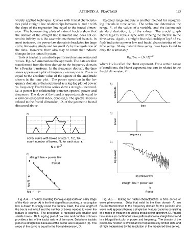
Fig. A.4.— The box-counting technique applied to an early stage Fig. A.5.— Testing for fractal characteristics in time series or
of the Koch curve. A) In the first step of box counting, a rectangular wave phenomena. Data that exist in the time domain A) are
box is drawn to snugly cover the feature. Next, the side length of Fourier-transformed to the frequency domain B); the periodic sine
the box is cut in half and the number of boxes needed to cover the wave in A) appears then as a single bar. Natural patterns consisting
feature is counted. The procedure is repeated with smaller and of a range of frequencies yield a broad power spectrum C). Fractal
smalle boxes. B) A log-log plot of box size and number of boxes time series (or continuous wave patterns) show a straight-line trend
provides a test of the fractal nature of the curve. Data from fractals in a bilogarithmic plot of power and frequency. The domain of the
plot on a straight line because of the power law in equation (1). The power-law relation is limited at low frequencies by limited data and
slope of the curve is equal to the fractal dimension, D. at high frequencies by the resolution of the measured time series.