Page 110 - Carrahers_Polymer_Chemistry,_Eighth_Edition

Molecular Weight of Polymers 73

Hc = 1 + 2Bc (3.17)
τ M w M w

Several expressions are generally used in describing the relationship between values measured
by light-scattering photometry and molecular weight. One is given in Equation 3.14 and the others,
such as Equation 3.18, are exactly analogous except that constants have been rearranged.

Kc 1 ( 2 )
+
+
= 12Bc Cc + ⋅⋅⋅ (3.18)
R M w
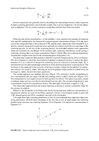
When the ratio of the concentration, c, to the turbidity, τ, (tau; related to the intensity of scattering
at 0 and 90 ) multiplied by the constant H is plotted against concentration (Figure 3.15), the inter-
o
o
cept of the extrapolated line is the reciprocal of M and the slope contains the viral constant B. Z is
w 0
directly related to the particle scattering factor, and both are related to both the size and shape of the
scattering particle. As the size of the scattering particle, the individual polymer chain approaches
about one-twentieth the wavelength of the incident light, scattering interference occurs giving a
scattering envelope that is no longer symmetrical (Figure 3.14(b)). Here the scattering dependency
on molecular weight reverts back to the relationship given in Equation 3.14.
The molecular weight for dilute polymer solutions is typically found using one of two techniques.

The first technique is called the dissymmetrical method or approach because it utilizes the deter-
mination of Z as a function of the particle-scattering factor as a function of polymer shape. M is
o w
determined from the intercept through substitution of the determined particle-scattering factor. The
weakness in this approach is the necessity of having to assume a shape for the polymer in a partic-
ular solution. For small Z values, choosing an incorrect polymer shape results in a small error, but
o
for larger Z values, the error becomes signifi cant.
o
The second approach uses multiple detectors (Figure 3.16), allowing a double extrapolation to
zero concentration and zero angle with the data forming what is called a Zimm plot (Figure 3.17).
The extrapolation to zero angle corrects for finite particle size effects. The radius of gyration, related

to polymer shape and size, can also be determined from this plot. The second extrapolation to zero
.
concentration corrects for concentration factors. The intercepts of both plots is equal to 1/ M w
The Zimm plot approach does not require knowing or having to assume a particular shape for
the polymer in solution.
Related to the Zimm plot is the Debye plot. In the Zimm approach, different concentrations of
the polymer solution are used. In the Debye approach, one low-concentration sample is used with
plotted against sin (θ /2), essentially one-half of the Zimm plot.
2
1/ M w
Low-angle laser light-scattering photometry (LALLS) and multiangle low-angle laser light-scat-
tering photometry (MALS) takes advantage of the fact that at low or small angles the scattering
particle factor becomes one reducing Equation 3.14 to Equation 3.16 and at low concentrations to
Equation 3.17.

+
+
+
Hc/t +

C
FIGURE 3.15 Typical simple plot used to determine 1/ M from scattering data.
w

9/14/2010 3:36:46 PM
K10478.indb 73
K10478.indb 73 9/14/2010 3:36:46 PM