Page 136 - Chemical Process Equipment - Selection and Design

108 FLOW OF FLUIDS
EXAMPLES 6.1&(continued)
~(cm) IO-~H~ xc Rea, v, The numbers in parentheses correspond to the break points on the
figure and agree roughly with the calculated values.
2.06 5.7 0.479 5635 114(120) The solution of this problem is based on that of Wasp et al.
4.04 22.0 0.635 8945 93 (109)
7.75 81.0 0.750 14,272 77 (1977).

dependence, pipe roughness, pipe fitting resistance, wall slippage, The Bingham data of Figure 6.6 are represented by the equations of
and viscoelastic behavior. Although some effort has been devoted Hanks [AZChE J. 9, 306 (1963)],
to them, none of these particular effects has been well correlated.
Viscoelasticity has been found to have little effect on friction in (Re,), = - :(; 1 - -x, + -$ :) ,
straight lines but does have a substantial effect on the resistance of (6.56)
pipe fittings. Pipe roughness often is accounted for by assuming that x,--
He
the relative effects of different roughness ratios &ID are represented (1 - x,)~ - 16,800. (6.57)
by the Colebrook equation (Eq. 6.20) for Newtonian fluids. Wall
slippage due to trace amounts of some polymers in solution is an They are employed in Example 6.10.
active field of research (Hoyt, 1972) and is not well predictable.
The scant literature on pipeline scaleup is reviewed by Turbulent Flow. Correlations have been achieved for all four
Heywood (1980). Some investigators have assumed a relation of the models, Eqs. (6.45)-(6.48). For power-law flow the correlation of
form Dodge and Metzner (1959) is shown in Figure 6.5(a) and is
rw = DAP/4L = kVa/Db represented by the equation
and determined the three constants K, a, and b from measurements 1 4.0 l~g,~[Re,~f~~-”’”)] $
on several diameters of pipe. The exponent a on the velocity -=- - (6.58)
e (n70.75
appears to be independent of the diameter if the roughness ratio
&ID is held constant. The exponent b on the diameter has been These authors and others have demonstrated that these results can
found to range from 0.2 to 0.25. How much better this kind of represent liquids with a variety of behavior over limited ranges by
analysis is than assuming that a = b, as in Eq. (6.48), has not been
established. If it can be assumed that the effect of differences in &ID
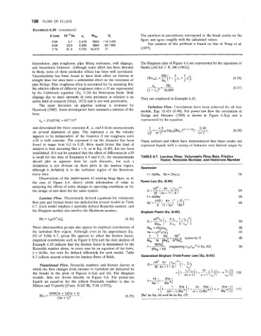
is small for the data of Examples 6.9 and 6.10, the measurements TABLE 6.7. Laminar Flow: Volumetric Flow Rate, Friction
should plot as separate lines for each diameter, but such a Factor, Reynolds Number, and Hedstrom Number
distinction is not obvious on those plots in the laminar region,
although it definitely is in the turbulent region of the limestone Newtonian
slurry data. f = 16/Re, Re = DVpP/p (1 1
Observations of the performance of existing large lines, as in
the case of Figure 6.4, clearly yields information of value in Power Law [Eq. (6.4511
analyzing the effects of some changes in operating conditions or for Q =-(->(%) 4n If”
nD3
the design of new lines for the same system.
32 3n+l
Laminar Flow. Theoretically derived equations for volumetric f = 16iRe’
flow rate and friction factor are included for several models in Table
6.7. Each model employs a specially defined Reynolds number, and
the Bingham models also involve the Hedstrom number,
Bingham Plastic [Eq. (6.4611
He = t0pD2/&. (6.54)

These dimensionless groups also appear in empirical correlations of
the turbulent flow region. Although even in the approximate Eq. He = toDzp/pi
(9) of Table 6.7, group He appears to affect the friction factor, 1 f He +- He4 (solve for f)
empirical correlations such as Figure 6.5(b) and the data analysis of _=__-
Re,
16 6Rei 3PRee8,
Example 6.10 indicate that the friction factor is determined by the fEP 96Re;
Reynolds number alone, in every case by an equation of the form, 6Rea + He [neglecting in Eq. (5)]
f = 16/Re, but with Re defined differently for each model. Table
6.7 collects several relations for laminar flows of fluids. Generalized Bingham (Yield-Power Law) [Eq. (6.4711
Transitional Flow. Reynolds numbers and friction factors at
which the flow changes from laminar to turbulent are indicated by
the breaks in the plots of Figures 6.4(a) and (b). For Bingham
models, data are Thown directly on Figure 6.6. For power-law
liquids an equation for the critical Reynolds number is due to
Mishra and Triparthi [Tram. ZChE 51, T141 (1973)],
1400(2n + 1)(5n + 3)
Re; = (6.55) [Re’ by Eq. (4) and He by Eq. (7)]
(3n + I)”