Page 102 - Chemical equilibria Volume 4

78 Chemical Equilibria
Δ
2
Hence: 0 k Δ g = 1 g 0 [3.49]
HM = k HM 1 [3.49a]
2
We can deduce from this that the two equilibrium pressures are such that:
Rln P = k R ln P 1 [3.50]
T
T
2
Thus:
ln P = k ln P [3.51]
2 1
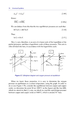
The y’y axis, therefore, is an axis of a linear scale of the logarithms of the
partial pressures, and thus a logarithmic scale of those pressures. This axis is
often divided into bars, in accordance with the logarithmic scale.

Figure 3.7. Ellingham diagram and oxygen pressure at equilibrium

When we know those properties, it is easy to determine the oxygen
pressure at equilibrium at a certain temperature, using the graph. In order to
do so (see Figure 3.7b), consider the equilibrium between copper and copper
oxide; we determine the point M (at 1000°C on the figure) and the line ΩM,
which we stretch to that y’y axis, on which we read the equilibrium pressure
-6
between copper and copper oxide at 1000°C, which is around 10 bars.