Page 114 - Chemical equilibria Volume 4

90 Chemical Equilibria
Coefficient β 2 may have a value of 0, in which case the equilibrium is
reached in the presence of an inert component of the solution – e.g. an inert
gas A 2.
3.5.1. Mode of representation

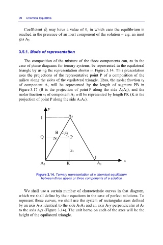
The composition of the mixture of the three components can, as in the
case of phase diagrams for ternary systems, be represented in the equilateral
triangle by using the representation shown in Figure 3.14. This presentation
uses the projections of the representative point P of a composition of the
milieu along the sides of the equilateral triangle. Thus, the molar fraction x 1
of component A 1 will be represented by the length of segment PB in
Figure 3.17 (B is the projection of point P along the side A 2A 3), and the
molar fraction x 3 of component A 3 will be represented by length PK (K is the
projection of point P along the side A 1A 2).

y

1 A 3

B x 1
Q N P

x 3
1
K A 1 x
A 2

Figure 3.14. Ternary representation of a chemical equilibrium
between three gases or three components of a solution

We shall use a certain number of characteristic curves in that diagram,
which we shall define by their equations in the case of perfect solutions. To
represent those curves, we shall use the system of rectangular axes defined
by an axis A 2x identical to the side A 2A 1 and an axis A 2y perpendicular at A 2
to the axis A 2x (Figure 3.14). The unit borne on each of the axes will be the
height of the equilateral triangle.