Page 128 - Chemical process engineering design and economics

112 Chapters

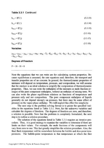
Table 3.3.1 Continued

hi^W) (3.3.13)

hi,2 = W) (3.3.14)
(3.3.15)

(3.3.16)

h 2L>, = f(T 2) (3.3.17)
h 2L,2 = f(T 2) (3.3.18)

Variables
m
y 2v,i - y 2v, 2 • y 2L,i - y 2L, 2 • 2v - rn 2L - T 2 - K 2jl - K 2;2 - h t - hi_i - h 1;2 - h 2V - h 2v,i - h 2V>2 - h 2L

Degrees of Freedom

F=18-18 = 0

Next the equations that we can write are for calculating system properties. Be-
cause equilibrium is assumed, the rate equations and, therefore, the transport and
transfer properties are of no concern. In general, the thermodynamic properties of
mixtures will depend on temperature, pressure, and composition, we will assume
that the mixture is an ideal solution to simplify the computation of thermodynamic
properties. Thus, we can write the enthalpies of the mixtures as mole fraction av-
erages of the pure component enthalpies, without an enthalpy of mixing term. We
can also write the phase equilibrium relations as functions of temperature and
pressure only and not composition. The pure component enthalpies of liquids
generally do not depend strongly on pressure, but there may be some effect of
pressure on the vapor-phase enthalpy. We will neglect this effect for simplicity.
The next step in the problem solving format is to prime the specified vari-
ables in the equations listed in Table 3.3.1. Next, list the unknown variables and
calculate the degrees of freedom. The degrees of freedom are zero, and therefore,
a solution is possible. Now that the problem is completely formulated, the next
step is to outline a solution procedure.
The solution of the equations listed in Table 3.3.1 requires an iterative pro-
cedure. Thus, it is good strategy to examine the variables to determine if there are
limits on their values. For example, the mole fractions of the components will
vary from zero to one. This fact greatly simplifies the solution procedure. Also, the
final flash temperature will lie somewhere between the bubble and dew-point tem-
peratures. The bubble-point temperature is that temperature at which the first

Copyright © 2003 by Taylor & Francis Group LLC