Page 290 - Chiral Separation Techniques

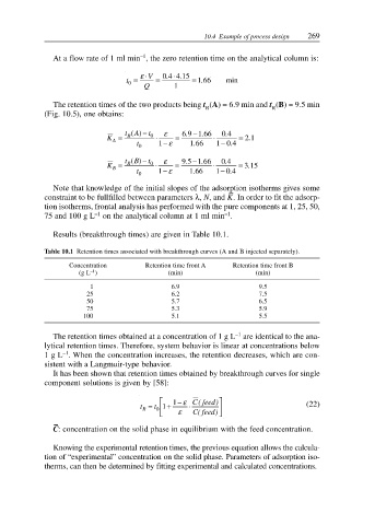
10.4 Example of process design 269

–1
At a flow rate of 1 ml min , the zero retention time on the analytical column is:
⋅
.
.
t = V ⋅ ε = 04 415 = 166 min
.
0
Q 1
The retention times of the two products being t (A) = 6.9 min and t (B) = 9.5 min
R R
(Fig. 10.5), one obtains:
tA − t ε
()
.
.
K = R 0 ⋅ = 69 −166. ⋅ 04 = 21.
A
.
− 4.
t 0 1 − ε 166 10
.
K = tB −() t 0 ⋅ ε = 95 . −166 ⋅ 04 . = 315
R
.
B
t 0 1 − ε 166 10.
.
− 4
Note that knowledge of the initial slopes of the adsorption isotherms gives some
–
constraint to be fullfilled between parameters λ, N, and K. In order to fit the adsorp-
tion isotherms, frontal analysis has performed with the pure components at 1, 25, 50,
–1
–1
75 and 100 g L on the analytical column at 1 ml min .
Results (breakthrough times) are given in Table 10.1.
Table 10.1 Retention times associated with breakthrough curves (A and B injected separately).
Concentration Retention time front A Retention time front B
–1
(g L ) (min) (min)
1 6.9 9.5
25 6.2 7.5
50 5.7 6.5
75 5.3 5.9
100 5.1 5.5
–1
The retention times obtained at a concentration of 1 g L are identical to the ana-
lytical retention times. Therefore, system behavior is linear at concentrations below
–1
1g L . When the concentration increases, the retention decreases, which are con-
sistent with a Langmuir-type behavior.
It has been shown that retention times obtained by breakthrough curves for single
component solutions is given by [58]:
 − ε
(
t = t 1 + 1 ⋅ C feed  ) (22)
R 0  ε 
(
 C feed) 
–
C: concentration on the solid phase in equilibrium with the feed concentration.
Knowing the experimental retention times, the previous equation allows the calcula-
tion of “experimental” concentration on the solid phase. Parameters of adsorption iso-
therms, can then be determined by fitting experimental and calculated concentrations.