
Page 139 - Circuit Analysis II with MATLAB Applications
P. 139
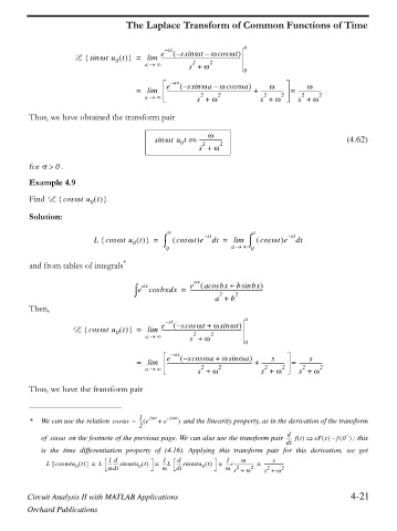
The Laplace Transform of Common Functions of Time
a
e – st s – sin Zt – Z Zcos t
L sin Ztu t ` = lim -----------------------------------------------------------
^
0
2
a o f s + Z 2
0
– as
Z
Z
= lim e s – sin Za Z – Zcos a ----------------- = -----------------
-------------------------------------------------------------- +
2
2
2
a o f s + Z 2 s + Z 2 s + Z 2
Thus, we have obtained the transform pair
Z
sin Ztu t ----------------- (4.62)
0
2
s + Z 2
for 0 V !
Example 4.9
Find L cos Zt u t ` 0
^
Solution:
f a
L cos Zt u t ` 0 ³ cos Z = t e – st dt = ³ lim cos Zt e – st dt
^
0 a o f 0
and from tables of integrals *
ax acos bx + bsin bx
e
ax
³ e cos bxdx = ------------------------------------------------------
2
a + b 2
Then,
a
–
st
-----------------------------------------------------------
L cos Zt u t ` 0 = lim e s – cos Zt + Z Zsin t
^
2
a o f s + Z 2
0
e – as s – cos Za + Z Zsin a s s
= lim --------------------------------------------------------------- + ----------------- = -----------------
2
2
2
a o f s + Z 2 s + Z 2 s + Z 2
Thus, we have the fransform pair
* We can use the relation cos Zt = 1 jZt + e – jZt and the linearity property, as in the derivation of the transform
--- e
2
d
of sin Zt on the footnote of the previous page. We can also use the transform pair ----- ft sF s – f0 ; this
dt
is the time differentiation property of (4.16). Applying this transform pair for this derivation, we get
1 d 1 d 1 Z s
L cos Ztu t = L --------- sin Ztu t = ----L ----- sin Ztu t = ----s----------------- = ----------------- 2
>
@
0
0
0
dt
Zdt
2
2
2
Z
Z
s +
s +
Z
Z
Circuit Analysis II with MATLAB Applications 4-21
Orchard Publications