Page 45 - Circuit Analysis II with MATLAB Applications

Other Second Order Circuits

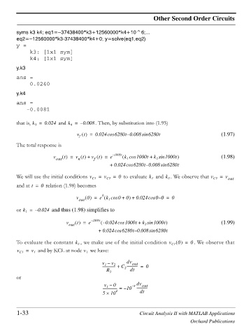
syms k3 k4; eq1= 37438400*k3+12560000*k4+10^6;...
eq2= 12560000*k3-37438400*k4+0; y=solve(eq1,eq2)
y =
k3: [1x1 sym]
k4: [1x1 sym]
y.k3

ans =
0.0240
y.k4

ans =
-0.0081

that is, k = 0.024 and k = – 0.008 . Then, by substitution into (1.95)
3
4
v t = 0.024cos 6280t 0.008sin 6280t (1.97)
–
f
The total response is

v out t = v t + v t = e – 1000t k cos 1000t + k sin 1000t (1.98)
n
f
1
2
–
+ 0.024cos 6280t 0.008sin 6280t
We will use the initial conditions v C1 = v C2 = 0 to evaluate k 1 and k 2 . We observe that v C2 = v out
and at t = 0 relation (1.98) becomes

0
v out 0 = e k cos + 0 + 0.024cos 0 0 = 0
0
–

1
or k = – 0.024 and thus (1.98) simplifies to
1
v out t = e – 1000t – 0.024cos 1000t + k sin 1000t (1.99)
2
+ 0.024cos 6280t 0.008sin 6280t
–
0
To evaluate the constant k 2 , we make use of the initial condition v = 0 . We observe that
C1
v C1 = v 1 and by KCL at node we have:
v
1
v – v dv out
1
2
--------------- + C ------------- = 0
2
R 3 dt
or
v – 0 – 8 dv out
1
----------------- = – 10 -------------
5 u 10 4 dt
1-33 Circuit Analysis II with MATLAB Applications
Orchard Publications