Page 55 - Circuit Analysis II with MATLAB Applications

Solutions to Exercises

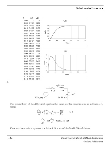
t v C (t) i L (t)
0.000 0 0 v C (t)
0.005 0.7191 2.206
0.010 2.6499 3.894 100
0.015 5.4977 5.155 80
0.020 9.0204 6.065 60
0.025 13.02 6.691 Volts 40
0.030 17.336 7.085 20
0.035 21.838 7.295 0
0.040 26.424 7.358 0.0 0.1 0.2 0.3 0.4 0.5
0.045 31.011 7.305 Time
0.050 35.536 7.163
0.055 39.951 6.953
0.060 44.217 6.694 i L (t)
0.065 48.311 6.4
8
0.070 52.212 6.082
0.075 55.91 5.751 6
0.080 59.399 5.413 4
0.085 62.677 5.076 Amps
0.090 65.745 4.743 2
0.095 68.608 4.418
0
0.100 71.27 4.104 0.0 0.1 0.2 0.3 0.4 0.5
0.105 73.741 3.803 Time
0.110 76.027 3.516
0.115 78.139 3.244
2.
i t
L
`
4 : 5H +
+ v t
C
100u t V 21.83 mF
0

The general form of the differential equation that describes this circuit is same as in Exercise 1,
that is,
2
d v R dv C 1 100
C
---------- + --- -------- + -------v = --------- t ! 0
C
dt 2 L dt LC LC
2
d v dv C
C
---------- + 0.8 -------- + 9.16v = 916
C
dt 2 dt
2
From the characteristic equation s + 0.8s + 9.16 = 0 and the MATLAB code below

1-43 Circuit Analysis II with MATLAB Applications
Orchard Publications